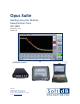
Opus Suite Building Acoustics Module Reverberation Time ISO 3382 User Guide – v1.3 2012-12-06 Compatible Hardware: Alto 6-Channel Concerto 4-Channel I-Track 6-Channel Soft dB Inc. 1040, Belvedere Avenue, Suite 215 Quebec (Quebec) Canada G1S 3G3 Toll free: 1-866-686-0993 (USA and Canada) E-mail: contact@softdb.
CONTENTS 1 Introduction ........................................................................................................................... 2 2 Compatible Hardware ............................................................................................................. 4 3 Opus Environment .................................................................................................................. 5 4 Quick Start........................................................................
1 Introduction Congratulations on your purchase of the Opus Suite RT-60 Module. The Opus Software Suite is a Sound and Vibration software. The current version contains six measurement modules: • SLM 4-ch module : 4-channels, Class 1 (IEC 61672 and ANSI S1.
• • • • • 1 Early Decay Time (EDT) Dynamic Clarity (C80)1 Central Time (Ts)* Definition (D50)* Only available with the automatic Schroeder method 3
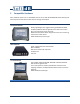
2 Compatible Hardware Every hardware option has an embedded state of the art Soft dB SR-MK3 DSP board allowing realtime and precise measurement with very low energy consumption. Concerto 4-Channel Alto 6-Channel I-Track 6-Channel Handy, lightweight, fully rugged military grade (MIL-STD-810F and IP67) tablet PC with anti-glare & anti-scratch touch screen All in one instrument (no PC required) WLAN communication allows using the Concerto as a monitoring station with remote access. www.softdb.
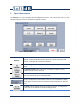
3 Opus Environment The Concerto unit comes equipped with the Opus Environment. This environment acts as a main interface that gives access to the different modules and tools. Modules The modules buttons will launch the associated module. When a module is opened, a license verification check is done. If no license is found for that module, a message will indicate the limitations. The File Manger button will launch the File Manager Utility (see section 9, p.
The Quit button will quit the application differently according to the hardware used. Concerto hardware: • Hold 5 sec to shutdown the unit. • Press and release to enter standby mode. Alto-6ch or I-Track hardware: • Press and release to close the application and return to Windows.
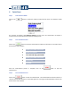
4 Quick Start Step 1 Click on the are: Select Measure Mode button to select the measure mode from the menu. The measure modes For purposes of example, select Manual Impulse from the menu. This mode does not require a sound source and can be performed simply by clapping hands. Step 2 Start the Measurement Click on the button to start the measurement. Follow the instructions in the status bar at the top of the main interface.
Step 4 Click on the Decay Spectrum Data Visualize the Measurement button to select the display from the menu. The available displays are: This display shows the time decay for a given frequency band or for the global. This display shows a selected value from each frequency band in a bar graph form. This display shows all values for all frequency bands in an array. Further information about each display is available in section 6.5, p. 12.
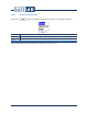
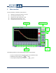
5 Main Interface The main interface is divided into five sections: 1) 2) 3) 4) 5) Measure controls (see section 6.1, p. 10) File info (see section 6.2, p. 10) Measure info (see section 6.3, p. 10) Menu bar (see section 6.4, p. 11) Display area (see section 6.5, p.
5.1 Measure Controls RUN/PAUSE/CONTINUE (Automatic mode) When the user clicks this button, the measurement process is launched. The RUN button then automatically becomes the PAUSE button. When the user clicks this button, the measurement process is suspended. The PAUSE button then automatically becomes the CONTINUE button When the user clicks this button, the measurement process continues from where it was suspended. The CONTINUE button then automatically becomes the PAUSE button.
be changed. This indicator displays the specified measure length. Clicking on this indicator launches the setup interface where the measure length can be changed. This indicator displays which reverberation indexes are met (i.e. if T10 is light on, it means that T10 was reached for every frequency bands and global). This control allows the software to automatically stop a measurement once the specified reverberation index is met. This control is only available in automatic Schroeder mode. 5.
Display Menu 5.5 Decay: This item sets the interface to display the time decay for a specified frequency band or global. Spectrum: This item sets the interface to display a specified reverberation index for all frequency bands and global on a bar graph. Data: This item sets the interface to display all the reverberation indexes for all frequency bands and global in an array. Display Area Data can be presented using one of three available displays: • Decay (see section 6.5.1, p.
5.5.1 Decay This display shows the response to a noise interruption or impulse. It also superimposes the curves used to evaluate RT values and the averaged successive responses. Spectrum Type Tab Curve Selection Time Decay Graph Frequency Selection Global / Frequency Selected Results Spectrum Type Tab Time Decay Graph Frequency Selection This tab switches between 1/1 octave bands 1/3 octave bands results. This graph displays the time decay curves for the selected frequency band or global.
5.5.2 Spectrum This display shows a selected result for each frequency band and global using a bar graph. Spectrum Type Tab Spectrum Bar Graph Global Bar Result Selection Cursor / Global Results Spectrum Type Tab This tab switches between 1/1 octave bands 1/3 octave bands results. Spectrum Bar Graph This graph displays the selected result for every frequency band. Result Selection These buttons are used to select the result to display on the spectrum graph and Global Bar.
5.5.3 Data This display shows all data for all frequency bands and global in a table form. Spectrum Type Tab Results Table Spectrum Type Tab Results Table This tab switches between 1/1 octave bands 1/3 octave bands results. This array displays all available results for every frequency band and global.
6 Setup Input Setup These controls allow selecting the input channel, the input type and the input range from drop down lists. Measure Mode This drop down list is used to select the measure mode. Measure Length This control is used to select the measure length in automatic mode. In manual mode, this control is unavailable. Averages This control is used to select the number of averages to perform. This control is unavailable in automatic Schroeder mode.
7 Measurement modes tutorials 7.1 Automatic Interrupted Noise This method evaluates the reverberation time by analysing the noise level decay occurring after a noise interruption. The noise interruptions are automatically generated using the internal noise generator. The result is a highly reproducible measurement that produces high precision results and allows a large number of averages. Step 1 Noise Source Set-Up Connect the Concerto output to the noise source using the appropriate cable.
Step 4 Stopping the Measurement The measurement stops when the specified number of Averages has been completed. However, the user can stop the measurement process any time by clicking the Step 5 button. Saving the Measurement The measurement is saved by clicking the button. When done, the current file indicator will display the current file name. 7.
Step 3 Running the Measurement Click the button to launch the measurement process. The noise will begin and the average number should increase periodically. You can follow the measurement process by displaying the Dynamic view on the Spectrum display. As the measurement proceeds, the dynamic should increase.
5) 6) Step 2 Select the appropriate Trigger Level4 necessary to detect the noise interruption. Click OK to return to the main interface. Running the Measurement 1) Turn on the external noise generator and adjust the volume to the desired level. 2) 3) Click the button to launch the measurement process.
The measurement is saved by clicking the indicator 7.4 button. Once complete, the current file will display the current file name. Manual Impulse This method evaluates the reverberation time by analysing the noise level time decay occurring after an impulse. The impulses are produced manually by clapping pieces of wood together or by bursting a balloon. Step 1 1) 2) 3) 4) 5) 6) Step 2 1) 2) Software Set-Up Click the button on the menu bar to access the setup interface.
Step 3 Adding More Average Iterations When an average iteration is finished, click the the same steps described in Step 2. Step 4 button. The process should go through Stopping the Measurement The measurement stops when the specified Average Number has been reached. The user can stop the measurement process any time by clicking the Step 5 Saving the Measurement The measurement is saved by clicking the indicator button. button. When complete, the current file will display the current file name.
8 Explorer Dialog File / Folder Operators Directory Path Shortcuts Directory Content Explorer Window Controls and Indicators File/Folder Operators Directory Path Shortcuts • • • • • Displays the path of the active directory. Accesses to common directories.
9 File Manager The File manager is used to perform most file operations: • • • • • Navigate the directory structure Create folders Rename files and folders Move or copy files and folders from one place to another Delete a file or a folder Although not very useful on a stand-alone computer, this manager is necessary on the Concerto, on which Windows explorer is unavailable.
Directory Path Displays the path of the active directory. Shortcuts • Desktop • My Documents • Computer When the File Manager is used on a Concerto, the shortcuts are linked to: Allows easy access to common directories. When the File Manager is used on a stand-alone computer, these shortcuts are linked to: • • Move/Copy Operators File/Folder Operators Directory Content Disk info Opus Root USB Device. Copies or moves a file or folder from a source to its destination.
Appendix 1: Concerto Hardware Connections Mic Stand 4 Inputs Loudspeaker Headphone Jack Power-on button 2 Outputs DC in ¼ 20 insert Second Battery USB port Battery indicator Right click 26 Enter Arrow keys
Power on/off Power-on Turn On Turn Off Press the trigger button located at the back of the unit This key has two (2) functions: 1. To turn the unit ON. 2. Start a measurement once the SLM Module is loaded After a few seconds, the Opus Environment Interface will appear. The stand-by mode allows fast load time. Stand-by • To put the unit on stand-by, click the Turn Off button.
Power Reset If the Concerto happens to crash and it is not possible to take back the control, a power reset might be necessary. To complete the power reset, the three buttons on the front of the Concerto must be used. Here is the procedure: Step 1 Press and hold the Function, Enter and Down Arrow button for 5 seconds until the Concerto shuts down Step 2 Wait 5 seconds and press the power button Step 3 Wait 5 seconds and press the power button a second time to restart the Concerto from a power reset.
Inputs and Signal Processing Specifications (Embedded Signal Ranger MK3 DSP Board) Texas Instruments TMS320C6424 DSP Processor 4 Inputs 2 Outputs 2 x (25-120 dBA or 30-130 dBA) + 2 x (25-120 dBA) Linear Range AC, DC, ICP (4 mA) Conditioning Physical (DAP Tech 9000 Tablet PC) Intel Atom E660T 1.3 GHz Operating system Storage Data Transfer 16 GB SSD USB Display 180 mm (7 inches) WVGA (800 x 480) Dimensions 230 x 185 x 60mm (9.0 x 7.3 x 2.
Appendix 2: 1/3 Octave Filters – IEC 61260 Class 1/ANSI S1.11 1/3 Octave Filters The 1/3 octave filters are computed at low-level in real time (at 48 kHz) on the digital signal processor (DSP) of the Concerto system. The filters comply with all requirements of IEC 61260 for Class 1. Frequency Range 20 Hz to 20 kHz. Filter Shape The following curve presents the filter shape test done for the 1000 Hz 1/3 octave band. The red and green curves represent the limits associated with the IEC standard (Class 1).
Shape Test Numerical Results at 1 kHz The following table presents the numerical results of the shape test at 1 kHz: Frequency (Hz) Low limit (dB) Measurement (dB) High limit (dB) 185.5 -inf -96.0 -75.0 327.5 -inf -85.1 -62.0 531.4 -inf -61.1 -42.5 772.6 -inf -28.2 -18.0 891.3 -4.5 -3.0 -2.3 919.6 -1.1 -0.3 0.15 947.0 -0.4 0.0 0.15 974.0 -0.2 0.0 0.15 1000.0 -0.15 0.0 0.15 1026.7 -0.2 0.0 0.15 1055.8 -0.4 0.0 0.15 1087.5 -1.1 -0.3 0.15 1122.0 -4.5 -3.
1/3 Octave Filter Linearity The linearity of the 1/3-octave filter has been measured for both ranges (low and high). The experimentation is done with an adaptor (ADP092) and an electric signal. The results in dB are for an input sensitivity of 50 mV/Pa. The maximum and the minimum linear levels are measured for each 1/3 octave band along with the noise floor. Filter Linearity (Low Range) Saturation Level Frequency (Hz) (dB) 120.5 20 Minimum Linear Level (dB) 39.5 Linear Dynamic Range (dB) 81.
Minimum Linear Level (dB) 27.0 Linear Dynamic Range (dB) 93.5 Noise Floor (dB) 12500 Saturation Level (dB) 120.5 16000 120.5 27.6 92.9 19.5 20000 120.5 28.3 92.2 19.7 Minimum Linear Level (dB) 51.5 Linear Dynamic Range (dB) 81.0 Noise Floor (dB) Frequency (Hz) Filter Linearity (High Range) Saturation Level Frequency (Hz) (dB) 132.5 20 17.5 7.3 25 132.5 49.2 83.3 5.3 31.5 132.5 47.1 85.4 2.0 40 132.5 44.2 88.3 7.9 50 132.5 41.8 90.7 9.3 63 132.5 39.1 93.4 9.
Minimum Linear Level (dB) 33.5 Linear Dynamic Range (dB) 99.0 Noise Floor (dB) 10000 Saturation Level (dB) 132.5 12500 132.5 34.1 98.4 25.2 16000 132.5 35.8 96.7 27.3 20000 132.5 37.1 95.4 27.7 Frequency (Hz) 23.5 1/3 Octave Filter Summation For this test, sine waves from 20 Hz to 20 kHz are measured with the Concerto system. For each sine wave the summation of the 1/3 octave filters is computed to form the following curves. The sine waves are electrical signals at 1 VRMS.
Summation Test (High Range Case) 0.5 0.4 0.3 Amplitude dB 0.2 0.1 0 -0.1 -0.2 -0.3 -0.4 -0.