FAST Survey Reference Manual
Copyright Notice Copyright 2010 Ashtech. All rights reserved. This manual is derived from the Carlson SurvCE Reference Manual, last revised Oct 13, 2010. Trademarks All product and brand names mentioned in this publication are trademarks of their respective holders.
THIS WARRANTY APPLIES ONLY TO THE ORIGINAL PURCHASER OF THIS PRODUCT. In the event of a defect, Ashtech will, at its option, repair or replace the hardware product with no charge to the purchaser for parts or labor. The repaired or replaced product will be warranted for 90 days from the date of return shipment, or for the balance of the original warranty, whichever is longer.
Table of Contents Installation 6 Using the Manual System Requirements Microsoft ActiveSync Installing FAST Survey Authorizing FAST Survey Hardware Notes Color Screens Memory Battery Status Save System 6 6 6 9 12 13 13 14 14 14 User Interface 15 FILE 27 EQUIP 75 Graphic Mode View Options Quick Calculator Hot Keys & Hot List Instrument Selection Input Box Controls Keyboard Operation Abbreviations 15 17 18 19 22 22 24 25 Job Job Settings (New Job) Job Settings (System) Job Settings (Format) Job Set
About FAST Survey 119 SURV 120 COGO 202 ROAD 224 MAP 283 Orientation (Instrument Setup) Orientation (Backsight) Orientation (Remote Benchmark) Orientation (Advanced Occupation) Orientation (Robotics) Store Points (TS) Store Points (TS Offsets) Store Points (GPS) Store Points (GPS Offsets) Stake Points Stake Line/Arc Stake Offset Elevation Difference Grid/Face Resection Set Collection Leveling Auto By Interval Remote Elevation Log Raw GPS 120 122 123 124 133 135 138 140 142 145 155 169 172 176 178
Tutorials 332 Instrument Setup by Manufacturer 357 GPS Utilities by Manufacturer 383 Troubleshooting 386 Raw Data 389 Tutorial 1: Calculating a Traverse (By Hand) with FAST Survey Tutorial 2: Performing Math Functions in FAST Survey Input Boxes Tutorial 3: Performing a Compass Rule Adjustment Tutorial 4: Defining Field Codes, Line/Layer Properties & GIS Prompting Tutorial 5: Standard Procedures for Conducting GPS Localizations Total Station (Geodimeter/Trimble) Total Station (Leica TPS Series) Tot
Installation This chapter describes the system requirements and installation instructions for FAST Survey. Using the Manual This manual is designed as a reference guide. It contains a complete description of all commands in the FAST Survey product. The chapters are organized by program menus, and they are arranged in the order that the menus typically appear in FAST Survey. Some commands are only applicable to either GPS or total station use and may not appear in your menu.
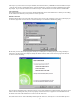
ActiveSync. If you do not have ActiveSync installed, insert the FAST Survey CD-ROM and choose “Install ActiveSync ”. You may also choose to download the latest version from Microsoft. After the ActiveSync installation starts, follow the prompts. If you need more assistance to install ActiveSync, visit Microsoft’s web site for the latest install details. Auto Connection If the default settings are correct, ActiveSync should automatically connect to the mobile device.
than once.) If successful, after you press Next, the following screen will appear and the connection will be made. In ActiveSync, you will then see the New Partnership dialog. Click No to setting up a partnership, and click Next. When you see the icon in the system tray, and it is green with no "x" through it, you are connected. Once you are connected, you should see the following dialog.
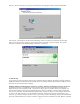
direct connections to the desktop computer” is checked. Note: When using FAST Survey’s Data Transfer option, you will need to disable Serial Port Connection (uncheck Allow Serial Cable). This is done in the Connection Settings in ActiveSync. This option must be enabled again in order to use ActiveSync. Installing FAST Survey Before you install FAST Survey, close all running applications on the mobile device. 1. 2. 3.
4. 5. On the next dialog, you must read and accept the FAST Survey End-User License Agreement (EULA). If you agree with the EULA, click "I accept ..." and then select Install. If you do not agree with the EULA, click "I do not accept ..." and the installation program will quit. The next dialog asks you to confirm the installation directory. Press Yes.
6. 7. At this point, the necessary files will be copied to the mobile device. A dialog will appear to show installation progress. You are given a final chance to check your mobile device. Click OK when you are ready, then click Finish on the desktop PC.
8. 9. On the Data Collector - Tap “Install” in the bottom left to install FAST Survey to the default location of “Device”. After tapping Install you will see an hourglass with a progress bar showing the installation progress. Once the Status Bar finishes on the data collector it will say “Software was successfully installed”. Tap OK in the upper right to complete the installation of FAST Survey.
4) Now go to the FAST Survey website at www.survce.com/ashtech to complete your registration via the Internet PLEASE NOTE: If you do not have access to the Internet, you may fax your company name, phone number, email address, your FAST Survey serial number, Hardware #1, Hardware #2 and the registration code to 606-564-9525. Your registration information will be faxed back to you within 48 hours. 5) Click on the “Registration Page” icon under Version 2.0/2.
Memory Memory is NOT an issue with newer data collectors running Windows Mobile. Please ignore this section of you have a Windows Mobile device. For all Windows Mobile users, there is no need to do any memory allocation. This section applies only to older, Windows CE devices like the early Rangers and Allegros. Memory on most Windows CE devices (excluding Windows Mobile), can be allocated directly by the user for best results when running or installing FAST Survey.
User Interface This chapter describes the general user interface features of FAST Survey. Graphic Mode Icons FAST Survey can be configured to show either the traditional letter icons or graphical icons for several functions. To set this option, go to the EQUIP tab, select Configure and toggle the "Use Graphic Icons" check box. This icon will Read a measurement (ALT-R). Total Station Only. This icon will Traverse to the measured point by advancing your setup (ALT-T).
display the Hgt/Desc prompt on Save (ALT-C). This icon will advance stake location incrementally to the Next point or station (ALT-N). stake data. This icon returns to the previous stakeout settings dialog where you can Modify the current design This icon allows the user to override the design Elevation (ALT-E). OK: This icon will accept the dialog. Back: This icon will return you to the previous dialog. Exit: This icon will return you to the main menu and dismiss any changes (ALT-X).
You can also pan the screen simply by touching it, then holding and dragging your finger or stylus along the screen surface. Pan is automatic and needs no prior command. View/Edit Points by Touch You can edit or delete any point by simply clicking on it graphically. In the Store Points command, clicking on a point also allows you to Re-Measure the point location, both in GPS and Total Station mode.
Intelligent Zoom: When selecting points "From Map" in commands such as Inverse or Stake Points, the "Intelligent Zoom" allows you to pick the point from the screen in a condensed area of points, and the program will auto-zoom allowing you to pick again and obtain the precise point that you want. If Intelligent Zoom is off, you would instead see a list of points and must pick from the list or return to the Map screen and zoom in closer using the Zoom + or Zoom Window options.
Hot Keys & Hot List The ALT key commands take the form ALT-C (Configure Reading) or ALT-N (Next Point). The ALT key and the subsequent "Hot Key" (“C” or “N”, as mentioned here) can be entered at nearly the same time or with any delay desired. If you press ALT and delay the entry of the hot key, you will see a text instruction: “Waiting for HotKey… Press Alt again to return”. A second ALT returns to the previous position in the program without executing any command.
ALT-I: Inverse. Does a quick inverse, and upon exit, returns you to the command you were in. Inverse is also accessible from the Helmet in the upper left of the screen, in many commands including Store Points. ALT-J: Joystick. Applies only to robotic total station. Takes you to the Settings option. ALT-J typically only functions if you are configured for a robotic total station. ALT-J will work from within data gathering commands, most stakeout commands (eg.
H I J K L M N O P Q R S T U V W X Y Z Interval Recording Help Help Inverse Inverse Sokkia Motorized: Joystick Calculator Calculator Feature Feature Code List Code List View Map View Map Offset Point Collection List Points Toggle Prompt for Hgt/Desc Store Offset Point Collection Help Inverse Joystick Calculator Feature Code List View Map Offset Point Collection List Points List Points Toggle Prompt for Hgt/Desc Toggle Prompt for Hgt/Desc On and Off On and Off Read Store Traverse Read and Store Store Tra
P Q R S T U V W X Y Z List Points List Points List Points Store Read Store Read and Store Store View Raw File Write Job Notes Exit to Main Menu Toggle Graphics/Text Mode Zoom to Point View Raw File Write Job Notes Exit to Main Menu Toggle Graphics/Text Mode (Helmet-Graph to return) Zoom to Point View Raw File Write Job Notes Exit to Main Menu Toggle Graphics/Text Mode (Helmet-Graph to return) Zoom to Point Instrument Selection The user can switch between current instruments using the Instrument Se
These extensions are automatically recognized for target heights and instrument heights, and within certain distance entry dialogs. Entries are not case sensitive. Formatted Bearing/Azimuth Entries Most directional commands within FAST Survey allow for the entry of both azimuths and bearings. Azimuth entries are in the form 350.2531 (DDD.MMSS), representing 350 degrees, 25 minutes and 31 seconds. But that same direction could be entered as N9.3429W or alternately as NW9.3429.
When ranges of points are involved, such as in stakeout lists, a dash is used. You can enter ranges in reverse (e.g.. 75-50), which would create a list of points from 75 down to 50 in reverse order. For example, in Stake Points, you could enter 75-50 for the point to stake, click "Add to List", then starting at point 75, stake 74, then 73, etc. by clicking N for Next. Survey Data Display Controls ANGLE The angle control will display the angle as defined by the current settings in Job Settings.
Right Down Left [Tab] [Shift+Tab] o Up/Down Arrows: Move to the next tab stop. Up [Tab] [Shift+Tab] o Tab: Move to the next tab stop. In Menus like Job Settings, Tab Right and Tab Left move through the tab headings (New Job, System, Format, Options, Stake) along the top of the dialog, while the right and left arrows move up and down through the options within each tab. Drop List o Enter: Selects the highlighted option within each drop list. o Right/Left Arrows: Move to the next tab stop.
Diff: Difference Dist: Distance El: Elevation Fst: Fast ft: Foot Fwd: Forward HD: Horizontal Distance HI: Height of Instrument. Horiz: Horizontal Ht: Height or Height of Antenna with GPS. HT: Height of Target.
FILE This chapter provides information on using the commands from the File menu. Job This command allows you to select an existing coordinate file for your job or to create a new coordinate file. The standard file selection dialog box appears for choosing a coordinate file, as shown in the next figure. Buttons for moving up the directory structure, creating a new folder, listing file names and listing file details appear in the upper right corner of the dialog box.
directory, as selected. Note: If you key in a coordinate file that already exists, it will load the file instead of overwriting it with a new file. The benefit of this feature is that you cannot accidentally overwrite an existing coordinate file from within FAST Survey. Job Settings (New Job) This tab allows you to configure how all new jobs will be created.
Job Settings (System) This tab allows you to define the units for the current job. Distance: Select the units that you want to use. Choices include US Feet, International Feet, and Metric. If US Feet or International Feet is selected, you have the option to display distances as decimal feet (Dec Ft) or Feet and Inches (Inches). This is a display property only and will not change the format of the data recorded to the raw file.
Note: The Projection selection applies primarily to GPS work and your localization file. It enables automatic calculation of grid to ground and ground to grid factors, for example (See Localization). However, the Projection can also apply to total station work. When you do any processing of your data within the Raw Data option (File Menu), there is an option "Reduce to Grid Coordinates".
Distance Observation Display: Options are Slope or Horizontal. This applies to the values displayed from total station readings. Slope Entry and Display: Whenever slopes are reported or prompted, you have the option to specify the default in Percent, Degrees or Ratio; however, some commands such as 3D Inverse will automatically report both slope and ratio and are unaffected. Station Display: This option impacts the display of centerline stationing, sometimes referred to as “chainage”. In the U.S.
Use Code Table for Descriptions: This feature activates feature code usage. If on, feature codes can be used to draw symbols and linework within specific layers. Special code icons also appear when "Hgt/Desc Prompt on Save" is on (within Equip-Configure). If "Use Code Table" is clicked off, use of feature codes is disabled and no linework or symbol drawing will occur. When clicked off, only the current descriptions used in the current job will appear.
Note: The above graphic display is non-default. In the Map screen, the normal display includes pull down menus. These can be disabled by selecting Preferences under the File menu. The screen shown below will appear with display options. The pull down menu format is recommended, since it contains the same graphic space, and also responds identically to keyed-in commands (such as PL for polyline).
Default Cutsheets to EXCEL (*.csv) Files: Stores Cutsheets in *.csv (EXCEL) format. Use Control File: The control file is used for selecting and using points that don’t exist in your current working file. Select File: You need to select a file for the control file. The chosen file appears, and will remain as the default control file, even when the control file option is disabled (in which case it is grayed out). Control files remain associated with active coordinate files.
Precision: Use this to control the decimal precision reported during stakeout routines. Store Data Note File: This option specifies whether or not to store the stakeout data in the note file (.NOT) for the current job. At the end of staking out a point, there is an option to store the staked coordinates in the current job. Note (.NOT) files are associated with points, so you must store the point to also store the cutsheet note. This additional data includes the target coordinates for reference.
Auto Descriptions This button allows you to configure the point description when you store points in stakeout. The very act of storing a staked point is optional. You can stake a point or a station and offset, but must click Store Point within the stakeout screens to actually store a point. If you do choose to store the point, the description is configurable. See image below. A user in Australia or Great Britain might want to change the STA for “Station” to CH for “Chainage”.
Alignments Tab (Applies to N for Next Station and all auto-incrementing of stations) Increment from Starting Station: For centerlines that start on an “odd” station such as 1020 (10+20 in U.S. stationing format), this option would conduct stakeout by interval measured from station 1020. So a 50 interval stakeout, instead of being 1050, 1100, 1150 would be 1020, 1070, 1120, etc.
Road Tab Next icon advances to: This defines how the "Next" icon will behave. It can advance to the next station or the next offset location. Stake Section File Locations: This instructs the software to stop at these critical locations even when they do not fall on the even station. Sections Include Catch Points: This instructs the software whether or not the design sections were extracted to the shoulder or the design catch location.
configurable items to report, and since commands such as Offset Stakeout, Point Projection and Stake Road do not stake out Point IDs, the program uses either the command name (CL for Stake Centerline, PP for Point Projection), offset reference, or template ID as the “design point name”. “RCurb”, for example, would be the name given to the design point in Offset Stakeout for top of curb, right side. This might lead to a variety of ID names for the design point.
offset is entered during stakeout, then two cut and fill results will appear for each point (useful, for example, for top and bottom of curb). List Points This command will list all of the points in the current coordinate (.crd) file. You can also edit any point in the list. If a Control File is active within Job Settings, Options, then you can also list and edit the Control File. The "From List" icon also allows you to recall points from both the current Job and the Control File job, if active.
Settings: Select the Settings button to customize the List Points display. The next figure shows the Settings dialog for List Points. Show Point Notes: Notes can be placed in any order on the list, or can be disabled, as shown above. (Only notes entered in response to “Prompt for Point Notes” or “Edit Notes” within List Points itself will display. Notes for GPS accuracy, time stamps and cutsheets, for example, appear in the raw file but not within List Points.
Note: If only the description value is edited, the raw data file will be updated without writing a store point record. If any other value that would change the point position is edited, the raw data file will record a store point record with the new position of the point. Add: To add a point, press the Add button. The Add Point dialog appears and you must enter the point ID, northing and easting. A store point record will be written to the raw data file.
Total station adjustments are conducted differently from GPS adjustments (Process GPS). If you wish to adjust your GPS first for control, and then calculate your total station traverse, first select Process GPS. Then use Process No Adjust, or Compass, as desired. Process Raw File Operations: Total Station, GPS, Reporting, Editing FAST Survey has made available four different types of raw file processing.
GPS Projection Tab: This tab, critical for GPS calculation, only applies for total station work when Reduce to Grid Coordinates is set on within the Total Station Tab. To change the active projection, go to the GPS tab under Job Settings. Redundancies Tab: This screen covers the handling of multiple measurements to the same point, known as redundancies. There are three options for Method: Use First, Use Last or Average.
Other Tab (for D&R Measurements): This tab contains settings for how to use direct and reverse (D&R) measurements. For the vertical angles, you can balance the direct and reverse measurements or use Direct-Only. When you have Foresight measurements and Backsight measurements (e.g. slope distance/zenith angles) between the same points (e.g. reciprocals) in Direct and Reverse surveys, you can Balance Foresight-Backsight measurements (apply reciprocals) or use the Foresight data only.
Angle Balance This method of processing applies an angle balance to the traverse lines when calculating the coordinates. The angle balance takes the angular error divided by the number of traverse lines and adjusts the angle of each traverse line by the calculated amount. The angular error is the difference between the angle balance shot and a reference angle. The program will prompt you to enter the traverse shot to use as the angle balance shot.
Next, the Reference Closing Angle dialog appears. Enter the bearing or azimuth of the reference angle, or define the reference angle with points by entering in the desired point numbers in the From Point and To Point fields. If using bearing or azimuth, enter the bearing in DD.MMSS format and then select the correct quadrant from the format field located at the bottom of the dialog. Once the reference angle has been defined, then the angular error display will update with the calculated angular error.
The angular adjustment applied to each traverse leg is also displayed, along with unadjusted angles and adjusted angles for each traverse leg. The adjusted coordinates are written to the coordinate file replacing the unadjusted coordinate values. Transit, Compass, Crandall Adjustments These methods apply the selected rule to the traverse lines when calculating the coordinates. After adjusting the traverse points, the sideshots can also be recalculated.
The reference point is specified by point ID or by entering the northing, easting and elevation of the reference point. The process results show varying information depending on selected options from the Process Raw Data Options dialog box. Reference Closing Point ID: The desired closing point number must be entered into this field. If the closing point does not exist in the coordinate file, the known coordinates can be entered into the North, East and Elevation fields on the dialog box.
Both lines and points can have attributes describing aspects such as material type, quality, age and date installed. You can create multiple feature code lists and each list can contain an unlimited number of codes. Each feature code consists of a short code, a longer description, a polyline toggle, and a polyline type setting. Point-type features can have symbols. All features can have associated prompting for GIS attributes.
Add a Feature Code Add: To add a code to the list, select this button. The Add Code dialog will appear. Select a Feature Code File Load: The Load button allows you to select a file to open or edit. Choose an existing file or enter a new file name to create a new Feature Code List. Feature Code List files have a *.FCL file extension. Edit an Existing Code Edit: If you wish to edit an existing code, double tap on the code or highlight it and tap Edit. It will appear in the Edit Code dialog.
Set Symbol: For Point entity types, symbols can be assigned, as an option. Symbols plot on the screen for quick reference and will export by .Dwg or DXF using the Map Screen, provided "Include Symbols" is clicked on. Layer: Symbols and linework can be assigned to layers, and will export to DXF or .Dwg files in the assigned layer. Even if office software is used to conduct field-to-finish, layers and distinct colors are useful for viewing points and linework while in the field.
Then for this new Feature Class (SWManhole), you can enter the 4 attributes. The result is shown below at left, with a typical attribute entry (use Add to create new entry) shown at below right. If you click "Add" in the "New Attribute" screen (below right), you can create a list of values to select from while in the field.
used, and there may be 6 options, with a default option. These can be set up, one time, by using the Add option within New Attributes. Once setup, whenever a fence is chosen, the attributes can be selected from a list. These attributes will be stored in the raw file and most importantly, will output to an ESRI Shape file (Map Screen, File pull down, Export SHP File).
Note in the dialog below, you can set when you are prompted for the line attributes (start vs end of line). This screen is found within Special Codes, Settings (button at top of screen in Special Codes). The "Use FCL Path to Store *.GIS" means that the folder used for the Feature Code File will also be the folder used for the *.GIS files that are made for each description with attributes. For example, if MH has attributes, a file MH.GIS will be created. If FH has attributes, a file FH.GIS will be created.
Special Codes: In addition to the codes that you add to the Feature Code List, there are some predefined code suffixes that you may use to end lines or start curves. For example, FL END could end the fence line, with “END” being a predefined special code. The need to append codes is one reason that the "END" button on your data collector is useful, to move to the END of the existing description so you can append a special code. You can substitute new codes for default codes, such that “..
CLO: Use this code to close a figure. This tells the software to close from the last point coded as CLO back to the first point of the figure. Note that after using a special code such as "CLO", appended with a space to the description code "BLD", that the program automatically removes the special code as it defaults the next description to "BLD". The "CLO" code also has the effect of ending the line and starting a new line. It only works with codes defined as 2D or 3D polylines.
JPN: Use this code followed by a point ID to create a new line segment between the current point and the entered point ID. RECT: This special code can be used in 2 different ways. You can take measurements to 3 sides of a building and on the third side, add the special code RECT, and the program will create a 4-sided building. Or you can measure two sides of a building and enter the distance right (RECT25) or distance left (RECT-20) to create the other, parallel sides. Both methods are illustrated below.
The OH and companion OV commands are flexible in that they can be entered after the first point measured, such as on point 121 or 122. NE: No Elevation. When a point is coded NE, it will not be used inside FAST Survey for contouring or use in volumes. However, if a 3D Polyline is drawn connecting between points, the elevation will be used. JOG: This powerful option allows you to hand-enter right-angle extensions of the last line segment.
On the first page, these codes going from top to bottom, starting at the left, represent start line, end line, close line, select active line (when multiple lines are being drawn with the same code), start curve, end curve, rectangle, and "more". When you pick more, the options are offset horizontal, offset vertical, smooth curve, select active line, join to point ID, no elevation, jog and more (return to first set of icons).
correct special codes that are active. Geopak also requires points to process linework, so it will not respond to the OH feature and the CLR feature, unless "Create Points for All Linework Elements" is turned on within Settings. (This option appears only if the program detects coding systems requiring the option). Otherwise, OH will create offset lines, for example, with no associated points.
Save Only One GIS Feature to the Stored Pt: When two codes are entered for the same point, seaprated by a space, and both codes lead to GIS prompting, only the first code will be used for the GIS prompts and stored attributes. Store Attributes (AT) to RW5 File: All attribute data will store at "AT" records in the raw file. For example, multiple attributes entered for a manhole might appear as shown below.
The 4 buttons along the top of the dialog represent Select Note, Clear Note, OK and Cancel. Create Points for All Linework Elements: When using OH or other codes such as RECT for Rectangle, this option creates a Point ID at all vertices of linework, whether surveyed or created by the software. Some office software packages, like earlier versions of Geopak, required point IDs to process coding. Points are increments sequentially from the last entered point.
You can survey points outside the pattern by simply entering a different code. The program will then resume auto-assigning the code based on the recognized pattern. Whenever Auto-Detect is on, it is advisable to review the automated code to be certain it matches what is intended. The button: "1.2.." in the HGT/Desc dialog gives you the option to: - turn ON/OFF auto-detect pattern. - check the codes that are making the pattern. - skip a code. - clear the codes that are making the pattern.
Even though point 79 was the newly measured point, point 14 is auto-updated to include BLD ST FL1 ST (start building, the original code and start fence line, the new code). The Line Details process therefore saves field measurement time and field coding time. Line Details, like Point Details, is a transparent or "context-sensitive" command. Simply pick the line or point, without issuing any command, and the options appear.
Reprocessing the Field Codes Using the command Field to Finish, found under the Tools pulldown menu in the Map screen, you can reprocess your field codes after editing any aspect of your point data. So if you left off an "end line" command, you can edit the point, change the description, and re-process the linework.
SDR33 transfer routine, then this option is designed to mimic that protocol. When an RW5 file is selected, it is automatically converted to a Sokkia RAW file and downloaded to the PC. When a CRD file is selected, it is automatically converted to a Sokkia RAW file with “08” records for points. This allows you to use and process the data in FAST Survey similarly to the data in the SDR33. You can also upload into the FAST Survey field computer Sokkia RAW files that contain point records.
3. 4. 5. If only the left side of the screen on the PC displays data, then you do not have a connection yet. Press the Connect button located at the bottom left of the file transfer dialog. The transfer program will respond with "Retrieving File List". Once the file list has been retrieved, the left side of the dialog box will show files located in the specified path on the PC, and the right side of the dialog will show the files located in the designated path on the remote.
Options: This command allows you to set various options for data transfer. The dialog shown in the figure below will appear. Com Port: You must select which com port on the PC to use. File Mask: You must select a file filtering syntax. Directory Sort: You must select how to sort the list of files. Display Special Files: Toggle whether or not you should see special files. Confirm Overwrite: Check this to confirm before overwriting files. Baud Rate: You must choose the baud rate for transferring data.
F2F Conversion: This converts the more thorough and detailed Carlson Survey field code file (for field-to-finish work) to the more simplified Feature Code List that runs in FAST Survey. The Feature Code List in FAST Survey handles Linework (on or off), Line Type (2D or 3D), Layer (= Code) and Full Text (Description). Send Points: The command allows for the sending of a range of points.
point IDs exceed that value, it is best to set Alphanumeric as the point ID type under New Job in Job Settings prior to importing. Geodimeter: For importing Geodimeter .OBS files. Trimble POS: For importing Trimble .POS files. CRD File: Allows you to import a FAST Survey CRD file into the current, active CRD file, and set the range of points to import. Note that this method can be used to move a subset of points from one CRD file over to another file, as shown below.
Coordinate Order: You must specify the output format for the ASCII file. There are seven different formats to choose from. The last field is always the description. The fields can be space, comma or tab delimited, and you can also separate the fields by a user-defined delimiter. Two of the options include quotes around the description field so that your descriptions can include spaces and/or commas.
Delete File This command allows you to remove any existing file from any directory to free up memory. This figure below shows the standard file selection dialog, where you can choose the file name to delete. Note: It is always a good idea to back-up your data by transferring it to a PC before deleting files. FAST Survey does not require you to back-up your data before deleting. Select the file you wish to delete from the standard file selection dialog box and pick OK.
Press Yes, if you wish to continue. You will be asked to confirm your file selection once more. Press Yes to accept the deletion of the file or files, or No to cancel the selection. Add Job Notes This command allows you to enter job notes as ASCII text. These notes are saved with the job in the raw data file. Exit This command will exit the FAST Survey program. The software presents the confirmation dialog. If you choose Yes, FAST Survey will exit and your data files are saved.
EQUIP This chapter provides information on using the commands from the Equip menu. Total Station The Total Station routine allows the user to configure their total station communication and operation settings. The tabs shown are configured based on the selected instrument (see specific instrument for details). It is recommended to go left to right through the tabs, from Current to Comms to Settings to Search, to ensure that all settings are correct, especially when first configuring a new instrument.
Load: This button will load all settings defined by the selected icon. Save: This button will save the current settings and allows the user to enter the name of new icons that will be created to represent the instrument settings. Rename: This button will allow the user to rename the selected icon. Delete: This button will remove the selected icon. Comms Tab There are 3 Comms options: Cable, Bluetooth, Radio. The Comms tab allows you to specify communication parameters for the data collector.
Port Number: You must select the COM port to use. This is the COM port of the data collector. Instrument (Bluetooth): FAST Survey can use Bluetooth to communicate only with instruments that have Bluetooth incorporated on them. The Instrument name is displayed when a Bluetooth connection is made. Baud Rate: Baud rate for data transfer by serial cable or radio. Parity: Parity setting is None, Odd or Even. Data Bits: You must select the character length setting.
are Standard (1.5 to 2 seconds), Fast, and Reflectorless. Referring to the graphic below, when storing points or staking points, your current mode of operation is displayed on the top line (eg. prism mode, locked on and tracking the target, measuring distances). Clicking the "little man" or distance tracking icon takes the program to the “No Distance” or “Tracking Only Mode” (no distance measurements, locked on and tracking target). Avoiding taking distance measurements will save battery usage.
30mm: Other manufactures (Sokkia, Seco). 40mm: Other manufacturers. Guidelights: When available, guidelights can be turned on or off and their intensity set by the user. They are seen from the prism viewpoint, and are valuable when running robotically from the prism, looking at the instrument. The field surveyor can see when he is lined up with the instrument by the appearance of the guidelights.
Manufacturer Setup Instructions For manufacturer specific information, please consult with the Instrument Setup by Manufacturer section. GPS Setup Both Base and Rover GPS are configured with Receiver and RTK in the same manner. Base GPS requires additional setup and is covered in the GPS Base section. GPS Rovers section covers the configuration of GPS networks and internet corrections. This section covers the common portion of the process, selecting the GPS equipment doing basic configuration.
Find Receiver Clicking the tools icon next to the right of Device proceeds to the Bluetooth Manager screen. This screen gives you the option to choose which GPS receiver you would like to connect to via Bluetooth. If you click Cancel, no Bluetooth connection will be established. Select a receiver and click the Bluetooth icon at the top of the screen, to connect. First time into this routine, no receivers will be listed. Select Find Receiver and you can add the connected receiver to the list.
Delete Receiver Highlight a Bluetooth Receiver and click Delete Receiver button to remove the device. You will be prompted before removing the device. Set Receiver PIN You can enter the receiver PIN by clicking “Set Receiver PIN”, and you can change the receiver name by clicking “Set Receiver Name”. The default PIN is usually 12345.
Trouble-shooting Note: Be sure the GPS receiver is turned on before trying to connect, and that you are within 30 feet of the receiver. If the user can’t see the device from the Bluetooth Devices program, it is not going to work in FAST Survey. The Bluetooth Manager works somewhat better with a passkey but it is not strictly necessary. Sometimes the Bluetooth registry settings don’t work correctly with an empty passkey. A pass key is the name the Bluetooth driver uses for a password.
The RTK tab is used to configure the GPS RTK communications. Device: This list contains the supported devices that deliver or receive RTK messages, such as a radio or IP modem. If an External Radio is selected, the user will need to specify the Port, Baud, Parity and Stop Bits that the radio manufacturer requires. For internal radios, FAST Survey will detect the proper settings. Network: This list allows you to configure and connect to various networks (e.g. NTRIP).
GPS Base for All RTK GPS Brands For all brands of GPS, the GPS Base button is the command that configures the base receiver for broadcasting GPS corrections to the rover. You must click the GPS Base button in while you are connected to the base receiver. The base needs a set of coordinates to use as its stationary position.
Latitude: N 42d21 ’28.35882” Longitude: W 71d08’12.87540” Elevation: 116.376 Continue with Base Setup? Yes No If you like the result, press Yes and continue on. You will then be prompted for the Reference Station Number. This is an “ID” that will store to the raw file and permit post-processing of the raw GPS data. A typical entry is 0001. The final prompt will say, Base Configuration Successful. Save Settings to File? Yes No Answering Yes will bring up an entry screen for the reference file name.
If it is a very accurate latitude and longitude, you will get the best results. Pressing OK leads to the option of store the base position as a reference file, similar to Read from GPS. Enter Grid System Coordinates: Requires you to enter the grid system northing and easting for the point that the base is occupying. This applies to any projection that you have configured, including U.S. state plane, worldwide UTM or any individual country or user-defined grid system.
From Known Position Options Previously Surveyed Point: This requires you to enter the coordinates, on the configured coordinate system, of a known, surveyed point. This will transform and localize to the local coordinate system, and optionally can be followed by rover-based localization. The known point must be found in the RW5 file in a form that includes its Lat/Long (a previous GPS measurement). This Lat/Long, just as with New Position options, is used to establish the base position.
When OK is pressed, you will be asked to load the associated “.dat” file, in a dialog similar to below: Read From File - Reads a previously saved base position file. All of the other methods of setting up the base let you save the base position at the end of setup. If you return to a site, set up the base in exactly the same position, use Read From File to use the same base position and you don’t have to re-align the rover: the old alignment is still valid.
which will change with each new set up, is entered back at the first set of dialogs. A message is displayed after successful configuration from a file. Only if you set the base antenna on the same horizontal and vertical position each day would the base antenna height remain fixed. If the base antenna height and x,y position is the same from day to day, then you do not need to do GPS Base each day. You would simply power up the base, power up the rover and start working in that case.
If a particular receiver model supports an internal modem or radio, meaning it is integrated into the receiver; those devices are shown first in the list. When an internal device is shown in the list, it means that model could have the device inside, but does not guarantee it. The user will have to know if the receiver was purchased with an integrated radio or modem.
To add a new base or network address, select in the Name field and replace the “” text with what you want to call the connection and fill out the Address and Port fields. Most modems support either an IP address (Ex: 192.202.228.252) or a URL address (Ex: www.basenetwork.com). UDP Direct: This works exactly like the TCP Direct option but uses UDP protocol instead of TCP. Most networks use TCP. NTRIP: This option is for base networks that support NTRIP protocol.
If you don’t like the name of the base supplied by the Broadcaster, you can change it to something else you prefer and FAST Survey will remember your preference but still ask the Broadcaster for the correct base. Select the base you want to use and press the green check box. You are brought back to the RTK tab with the base you selected as the current Base ID. You can change the Base ID in the RTK tab without going back to the NTRIP Configure button.
SpiderNet: Networks that require that a GPUID message be sent to the network should use the SpiderNet option. The SpiderNet Configure window comes up when the Configure button to the right of the SpiderNet option is pressed. Add a new network by selecting in the Name combo box and typing in the name of the network and filling out the other fields. If the User Name and Password fields are left empty, the GPUID message is not sent to the network.
Press the Configure button to the right of the Data Collector Internet option. Select the COM port on the data collector that is connected to the RTK port of the GPS rover receiver. It cannot be the same port that is used to control the receiver and is selected in the GPS Rover Comms tab. It may be a serial port or a BT port with a connection that has already been established. After selecting the port and pressing the green check to accept the input, select the network type in the RTK tab.
Common GPS Utilities Reset Receiver: This command performs a soft reset of the GPS receiver. Soft resets will reinitialize the receiver like a power cycle. Soft reset does not delete the memory. Factory Reset or Hard Reset: This command will erase the memory of the receiver and restore the setting to a factory settings. Power Off Receiver: This will power down the receiver. Save Settings to Receiver: Stores receiver settings to internal memory. Beep Off: Turns off the receiver alarms.
GPS Utilites by Manufacturer Setup Manufacturer specific information is available in the GPS Utilities by Manufacturer section. Configure (General) This tab allows you to select settings and preferences that apply to observations taken in the field. These options remain set from job to job. If an option is not applicable, it is grayed out. Configure is accessible from within any routine where the C or Configure Icon is present. These options can also be accessed by pressing ALT-C on the keyboard.
Store Fixed Only: When enabled, only data gathered in the fixed (locked) status will be stored to the point file. If you attempt to store data when the receiver is not fixed, a message will appear stating, "Position is not fixed! Continue storing?" The program will prompt to store the point anyway. This allows for overwriting the Store Fixed Only option without having to go back to the Configure menu.
No. of Readings to Avg (TS & GPS): Specifies the number of readings that will be taken and averaged on each observation. Values between 1 and 9 are accepted for Total Stations and 1-999 for GPS. If the tolerance is exceeded between readings, a warning screen will appear. Note: The Num Dist Readings setting does not apply to Manual Total Station mode. In this mode, you can use the Calculator to average distances. When prompted for Slope Distance, enter ?” “ to bring up the calculator.
Method Options: North-South, East-West: When total stations are used, the direction to go in stakeout can be North-South, East-West. For instance, the program might advise, "North 3.582, East 1.917." This method is better suited to GPS work and is subject to having a sense, in the field, of the north direction. In-Out, Left-Right: Nearly all surveyors choose this method.
D&R: The user can choose to measure direct and reverse readings for backsight, traverse, resection, topography, or stakeout routines. If the user measures direct and reverse for the backsight readings, all foresight readings that also are recorded direct and reverse will be recorded and computed as angle sets.
Projection: If you click the arrow to the right of the current projection, you can select from a list of projections that you have previously created. But to select a projection that you haven’t previously used, choose Edit Projection List. Convert WGS84 to NAD83. Most base stations in North America broadcast NAD83 positions. Turn this option on when a North American base station is transmitting WGS84 positions. Leave this option off for all other situations.
calculation. You may select between the Clarke 1866 ellipsoid and the WGS84 ellipsoid. New Zealand: You may select between “NZGD2000” and “NZGD49”. Both use the Transverse Mercator calculation. NZGD2000 uses the GRS80 ellipsoid. NZGD49 uses the International 1924 ellipsoid. You may specify a Meridional Circuit with either datum. To select the circuit, press the Define button. You will see a pull-down list with all Meridional Circuits as well as the option to pick None.
If the values you have are “from WGS84”, simply reverse the sign of each value (positive becomes negative and vice versa). You will need to save the system to a file. You may save the system to a “.sys” file or a “.csl” file. Sys files contain only one system definition. Csl files contain multiple system definitions. Both files are ASCII text files using OpenGIS WKT (Well Known Text) format.
C & R (Curvature and Refraction): This option applies only to total station configurations and will be unavailable when your instrument is configured to any GPS option. This factor causes an adjustment in distance measurement. Effects are negligible except over long distances. It is recommended that this toggle be enabled, except in those very rare cases where the instrument factors in curvature and refraction.
must directly type in the desired Ground to Grid Factor. GPS Tab The GPS tab is where you define the RTK methods, geoid file, and GPS scale factor. The geodi RTK Method (Transformation Types): The transformation can be by plane similarity, rigid body, or seven-parameter Helmert methods. Plane Similarity and Rigid Body both use a best-fit least-squares transformation. The difference is that the rigid body method does a transformation with a translation and rotation, without scale.
case, the scale factor is fixed by the localization itself, and is the inverse of the value appearing in localization, because within Units, we display the “ground to grid” number, whereas in localization, we display the “grid to ground” multiplier. For base or one-point rover localizations, Read GPS applies. After converting the LAT/LONG from the GPS to the state plane coordinates and computing the grid and elevation factors, the Scale Factor is applied as the final adjustment to the coordinates.
5. 6. 7. 8. 9. 10. 11. 12. 13. 14. 15. 16. 17. 18. 19. Run Carlson SurvCE on the handheld device and select Data Transfer from the FILE tab. From within the Data Transfer dialog, select the SurvCADD(Carlson Civil)/Carlson Survey Transfer option. Leave the data collector waiting for communications as shown by the resulting File Transfer dialog. Launch either Carlson X-Port or SurvCOM from your desktop computer.
Add Method 2--Enter Latitude/Longitude: This allows you to hand-enter known geodetic coordinates for the local position. The elevation should be the ellipsoid elevation in the current job units if a geoid model is not applied. If a geoid model is applied, then the elevation should be the orthometric elevation in the current job units. This method allows manual entry of a localization file without occupying points in the field. Note that you do not enter the decimal point for decimal seconds.
Note that in this example, it takes three horizontal control points, active “H On = Y” to get horizontal residual results, and four vertical control points, active “V On = Y” to get vertical residual results. You can employ trial and error to remove different points from consideration both vertically and horizontally and watch the residuals of the remaining control points improve or degrade.
your goal is to work on the specified state plane, UTM or other grid coordinate system, and you are planning to use a one-point localization, then the scale factor should be set to 1, unless you are trying to match “ground” coordinates, where the coordinates are “true north” but not “true scale”. In all other cases, matching ground coordinates with GPS is best accomplished with a multi-point rover-based localization.
point, it is still possible to recalculate all the field shots taken earlier from the less accurate base. To do so, follow the procedure outlined below. 1. Store the Base Point (Reference Tab in the Monitor screen). 2. Add a point to the now-empty Localization File. For the local point, enter the grid system coordinate computed by OPUS or other program. For the geodetic Lat/Lon point, review the raw file and select the point you stored for the base. 3. Reprocess the raw file through the localization.
SATView: Under the SATView tab, the spatial orientation of the satellite constellation is shown. You can also see if the satellite is rising or falling in the sky, by the associated arrow. Click on any satellite number to see individual satellite details, including the precise signal/noise ratio. You can also toggle satellites on and off if supported by the GPS. If a satellite is turned off, it displays with a line through it within the Signal/Noise Ratio graphs.
Check Level (Total Station) This feature is only available on instruments that provide information from electronic compensators. It allows the user to Check the level of the instrument from within the software. Tilt T: Shows the compensator value. Tilt L: Shows the compensator value. Tolerances This command allows you to set operating tolerances for the collection of points.
H. Obs: This specifies the horizontal observation tolerance as an angle field. A tolerance of zero is not allowed. V. Obs: This specifies the vertical observation tolerance as an angle field. A tolerance of zero is not allowed. Edm tol (mm): EDM fixed tolerance in millimeters specifies the EDM error that is independent of the length of the line measured. Stakeout Tol: This specifies the maximum difference between the target location and actual staked point.
Peripherals A Peripheral is a device that must be used in tandem with a GPS receiver or a total station. Peripherals can all be configured from the Peripherals menu under the EQUIP tab. Lasers, Light Bars, and Depth Sounders are all supported as peripherals. If a peripheral is not currently in use, it is strongly recommended that you deactivate it, so it does not slow down other operations.
2. 3. A progress window should pop up, indicating that FAST Survey is ready to read from the laser. Aim the laser and fire at a target point. Keep firing until your laser returns a valid reading, and the progress window disappears. To test whether your shot was successful, verify that the values on your screen correspond to the values on your laser’s internal display. Note that not all lasers return azimuth and vertical offset data, in which case this information will have to be entered manually.
Laser Impulse manual for instructions. Sokkia Contour: Make sure your Sokkia Contour’s baud-rate agrees with those specified in FAST Survey. Consult your Sokkia Contour manual for instructions. MDL LaserAce: Using FAST Survey, you can use the LaserAce, but should configure your peripherals screen to Impulse (CR400). Using the MDL selection will invert the inclination. Use 9600 baud rate. Use a Topcon/Sokkia data cable (not a Nikon cable!).
To activate the light bar, follow these steps: 1. Plug in the light bar to any of your device’s unused COM ports and turn it on. 2. Enter the Peripherals menu, and select the Light Bar tab, as shown above. 3. Check Active 4. Select the Type of light bar you are using. 5. Set the Grading Tolerance to the maximum permissible deviation from the target path or elevation. 6. Specify the Port the Light Bar is plugged in to.
SURV This chapter provides information on using the commands from the Survey menu. Orientation (Instrument Setup) The instrument setup dialog is displayed upon entering every active survey routine, unless "Prompt for Total Station Setup" is clicked off within Configuration. You also go directly to the Orientation screen whenever you click the tripod icon in all survey and stakeout routines.
When simply confirming the backsight information, if the OK button (green checkmark) is active, you can simply press Enter or click OK to move on to the active survey screen. If the OK button is grayed out, that means the program has detected a new occupied point (or the first one of the survey). Then you must click the Backsight screen and take an angle and/or distance measurement to the backsight.
icons to the right. You can also click the station and offset icon, as with the occupied point. A backsight point ID is required, even if you choose to enter an azimuth or bearing only. Backsight Bearing or Azimuth: This displays the bearing or azimuth between the two entered points, when both points have coordinates. If Angle Type, in Job Settings, is set to bearing, then a backsight bearing will appear. If set to azimuth, then the backsight azimuth is shown.
read 190 degrees from the instrument. This is useful in underground mine surveying because it ensures that the readings displayed by the total station always refer to true azimuth. Some surveyors are “azimuth” surveyors and others prefer “set zero”. Use Current (Do Not Set Angle): Uses whatever direction reading is already in the instrument. Set Angle and Read: This button will set the horizontal angle and read the distance to the backsight.
Read: You have the option to transfer the elevation from a single benchmark by taking a reading on it, any number of times, in any face. You may also use multiple benchmark points, any number of times, in any face. If you turn on Direct and Reverse for Resection in Configuration, Sets tab, robotic instruments will perform a D&R automatically for remote elevation readings as well. Results: The readings taken on the benchmark are reported in the Results dialog.
Although standard backsight procedure may be to take one or more readings to a single backsight, the Advanced Occupation command allows multiple readings to be taken for the backsight, to points identified in advance, leading to a 'best fit" backsight orientation computed by least squares methods. Consider the graphic below, showing a proposed occupied point (tripod) and three known point IDs as originally surveyed and precisely located based on a due North backsight.
(or in Resection). The radio tower points will be used only for their north and east coordinates. The Advanced Occupation command can even be run from a file containing no coordinates, assuming backsight points can be referenced from a control file. Begin by selecting the command Store Points in the Surv Menu, establish point 1 as the occupied point, 2 as the backsight and enter the correct target heights (0 for the radiotower point 2). Then click to "Occupation".
Entering point 2 as a target leads to presentation of the coordinates for 2. Since this is an "angle-only" measurement, turn off the slope distance "SD" option and turn off the "Use Known Elev" option. The "Zenith Angle" option is also irrelevant but can be left on or off. The goal of Observations is to load in advance all targets that will be used for the multiple backsight measurement. So if in this case, our goal is to backsight control points 2, 3 and 4, we would select those point IDs.
In this example, we would add points 3 and 4. Note that for point 4, a target height of 2 meters will be used, and the slope distance reading and elevation of point 4 will also be used in the calculation. When distance measurements are involved, the prism offset can be entered distinctly for each measurement. When the entire list of targets has been entered, you then select the target to measure first (eg. point ID 2) and then tap "Measure".
You will be prompted to the turn to the target in direct face, and take the reading. Assuming you set zero on the instrument to the backsight to point 2, the following measurements may be entered: After the first measurement is taken, you are asked if you wish to complete the set to the rest of the points. Click Yes. Then you can take readings to the remaining points, as shown below: When all direct measurements are taken, you will be asked to continue the measurements in reverse face.
Here, you will either be led to the results screen showing the successful calculation, or it will report, "Unable to retrieve solution results". In the case above, the computed results are shown below: Note that the "averaged" backsight orientation is 52.9704, although by setting 0 to point 2, the mathematically computed backsight reading would be 52.9703. An added feature of the Advanced Occupation routine is the calculation of the occupied point coordinates.
Apply Collimation: Leads to a report on the collimation of the total staiton instrument provided that both direct and reverse measurements are taken to the same foresights. Apply Refraction Correction: This option should be selected only if the instrument itself does not automatically apply refraction correction in the reported readings.
After cylcing through all targets and being prompted for reverse readings (optional), you are returned to the target list. If you highlight a target and click Measure again, you are in effect launching another set of readings. You will be prompted as shown below: After completing a set, if you click Measure for measurements, you can accumulate multiple readings which can vary from target to target, depending on whether you choose to skip certain target readings, do direct only, etc.
the following prompt, after which it announces "Operation Complete. Angle Set." For any reading, within the Edit option, you can delete aspects of the reading. If you want to delete the entire entry in the list of targets (for example, you want to delete target 4 from the list), then select 4 and click Edit, which brings you to the screen in the lower left, then click the eraser icon at the top of the screen and click on "All" (lower right).
Arrow Keys for Joystick ALT-J will take you directly to the robotics dialog from elsewhere in the program. The arrow-key motion is sometimes referred to as the Joystick Speed. Leica: Tapping once in the direction you want (e.g. up) causes the instrument to move slowly, two taps medium, and 3 taps fast speed. Tapping the other direction (e.g. down) stops the movement. Geodimeter/Trimble: Press the arrow key once. After a small delay, the instrument will move an incremental amount.
Settings: This button leads to a series of settings screens that allow you to dial in the speed of motion, range of motion, and other factors governing arrow-key driven movement and automatic searching. Store Points (TS) This command is designed for total stations and manual entry. It is the principal data collection routine with total stations. Store Points interacts with numerous settings, including the feature codes that will draw line work.
Enter saves the measurement immediately. If you do a Read, you can review the data within the Text view. If you re-enter the rod height, it re-calculates the Z elevation of the measured point. As you enter the description, a pulldown appears of your Feature Code List or previously entered descriptions. As each letter is entered, such as "e" for edge of pavement, every description beginning with "e" or "E" appears, enabling quick selections.
Note: FAST Survey is designed to produce a 1 keystroke point store, by pressing Enter. If you experience more prompts storing a point, it is because you have certain settings active that cause additional prompts.
following the prism but not tracking (taking distance measurements, showing position of prism on the screen). Standby: Stopped in the last position it was in and ready to resume Tracking. Searching: Looking for the prism (shows an hourglass). No Data: Brief mode between losing the prism and beginning an automatic search.
2-reading option), and a new point ID will be stored. Within Offset, whenever you do a fresh, new Read, you will substitute the new reading for the one previously stored in memory. If you have no previous measurement, a new Read is required within O for Offset. So in summary, you can offset something you've already measured, or you can take a fresh measurement (typical method), using O for Offset. The total station Offset command must be selected each time it is used.
to use the Offset button in Store Points, and then the Point method. You do a Read and enter 0 for all offsets, then Store. Then change the description and tap Store again (no additional Read is necessary), and a second point with a different description (or rod height, or offset) is stored. Some office software programs require distinct readings on the same point to process multiple descriptions, in which case the use of Offsets to store multiple readings with one field measurement is recommended.
For GPS, coordinates, status (Fixed, Float, Autonomous) and HRMS and VRMS accuracy estimates are displayed at all times. The icons at the left are for zooming and panning. From top to bottom, they are: zoom extents, zoom in, zoom out, zoom window, zoom previous and point display control. If you prefer to work in a pure text screen, without graphics, you can tap the helmet icon and select TEXT. The following dialog will appear.
Offsets This icon leads to Offset reading screens with options for keyed-in offsets as well as offsets taken by laser devices. These devices can measure distance only or distance and azimuth (ALT-O). See Store Points (GPS Offsets) for more details. Configure This icon will take you to the Configure dialog, also found on the EQUIP tab. From this dialog you can set the number of readings to average, specify to only store fixed readings, and turn on or off the Hgt/Desc prompt on Save (ALT-C).
offset values as show below. The azimuth can either be specified with respect to north, or with respect to a specified point. Current GPS coordinates are shown at the bottom, and can be updated via the Read GPS button. When all necessary data has been entered, you’ll be able to store by tapping Store, or preview the point you’re storing by selecting Map, or Results.
Results: Before storing, you can preview the data by selecting the RESULTS tab. If valid data has been entered in the LASER or OFFSET tab, the result will appear as shown below. In this window, you can also change the GPS antenna height, or specify a vertical difference for your target point. You can also specify the point ID and description for the point that will be stored. Offset by Intersection Use Offset by Intersection to calculate a point based on two GPS positions and two distance offsets.
Offset: Under the Offset tab, press Read Point 1 to read the first point from GPS. Repeat this process for the second point. The GPS antenna height used for each GPS read can be adjusted individually by editing the HT fields. Now enter the offset of the point you would like to store, or press Read Dist to read it from a laser. Finally, specify the direction of your offset, and switch to the RESULTS tab to see your solution.
A read function is required to update the directional display information. You should see your points in the map with an icon showing your target location (the circle with the X inside). Measurements are taken typically by pressing Enter. Enter also transitions automatically from the Stake Points entry screen to the Stk Pt measurement screens above. Point Stakeout can be conducted without touching the screen, using the Enter key and entering point IDs using the keyboard.
accessible through the tripod icon or C for Configure), you can turn on "Turn to Horizontal" in Stakeout. If this is turned on, the instrument will turn to the target point automatically. If "Turn to Vertical" is also on, and the correct target height is entered, the instrument will turn to both the horizontal and vertical position of the target. Do not use "Turn to Vertical" if the elevation of the target point is 0 or not accurate. Point ID: This is the point which you are staking.
N for Next (Increment Up or Down) On some projects, you may find that it is more convenient to stakeout points in descending order. This can be accomplished by going to File, Job Settings, Stake tab, and switching to increment in descending order. If Increment ID Down is set, then N for Next would go to point ID 330, then to 329, etc.
Right/Left Distance, Azimuth and Distance, or North/South East/West Distances. The cut or fill is the elevation difference between the point read and the point being staked. Normally, you take a shot simply by pressing Enter. After a total station shot is taken, you will see your “In-Out” distance to the target point. For total station stakeout, the direction of the reference is shown by a little arrow in the lower right of the screen.
Pressing OK (which optionally will Store Point if enabled) will return to the Stakeout Points dialog to select the next point for staking. If the Use Control File option is set under the Job Settings, you have the option of staking control file points. If you enter in a point number to store that is the same as a point number in the control file, the point in the control file will remain unchanged. It will only modify the point in the current coordinate file.
the instrument. When the lock is shown, the instrument is locked onto the target. If you press the lock icon, it will switch to Search mode. For Tracking to occur (distance measurements leading to known target position shown by triangle), the instrument must be locked. If the binoculars are shown, the instrument is in Search mode, and pressing the Search icon (binoculars) will start the search process, with the window of the search determined in Settings.
Using the graphic screen selection of points, you also have the ability to see the last point picked. So if you are selecting a series of tightly-spaced "endpoints" of lines, using the endpoint snap, you can see your last point, and pick the next one, by reference. The last point selected is shown by a pencil, so if you are staking endpoints right-to-left, you select the next point shown illustrated here by an arrow.
Some of the more useful commands to access, at any time, are Inverse (obtain 2D and 3D distance between points), View Data (review the cut and fill "cutsheets" and review and edit the raw file), Points (review the coordinates in the job file, delete and edit as desired) and Freeze Points (to freeze the point numbers and reduce clutter on the screen).
There is a third mode for the Maximized Map which is called "Measurements". With this mode set, and running a robotic total station, the larger map appears as shown below, with the current measurement data presented on a second line.
The instructions given are controlled by the settings in Configure, View Pt tab. In this case, the instructions are In-Out, Left-Right facing the instrument from the perspective of the rod or prism. This would be a typical configuration for running as a one-man crew working from the rod and facing a robotic total station.
Stake Station Interval is clicked off, the program reports the station and offset of measured points and for your current position (GPS and robotic total stations), and does not prompt for a target station,offset and interval. It leads to fewer screens and does not include the "Point on Line" and "Point on Arc" options, which appear specifically in the Stake Station Interval dialogs.
instructions you receive in stakeout. You should review the settings in the Stake tab under Job Settings, as well as the Configure option within Equip before staking. The dialogs are varied slightly with respect to total station or GPS equipment. Both types are documented here, illustrating the differences between the dialogs. Stakeout by Define Line also has a Point On Line tab that enables, in total station mode, staking of the intersect with the specified line on the current line-of-sight.
Stake Station Interval Off For standard total stations, a measurement must be taken (Enter key or R for Read) to see the Station, Offset and Cut or Fill. With total stations, dashed lines are drawn from the instrument to the backsight, to the current point being measured, and perpendicular to the defined line.
Stake Station Interval On Define Alignments (Horizontal) Stakeout Centerline only requires a horizontal alignment, but you have the option to specify a vertical alignment which will lead to cut and fill results as well. Additionally, you can specify a reference alignment. This feature allows you to stake the offset off of one alignment (e.g. curb) and report the station of a reference alignment (e.g. centerline).
Reverse Alignment Direction: After selection of a polyline, you can use the "Reverse" icon to reverse the direction of the alignment, ensuring that it increments the stationing in the desired direction. This feature is found throughout the software where horizontal alignments are selected from the screen. In the case of File-based or Point-based alignments, the direction is defined by the file or point order itself.
With Stake Station Interval On, the alignment selection screen continues into the Station/Offset screen where you select your station and offset to stake out. Using Define Alignments, the Point on Line option becomes Point on CL in the screen that follows. With both horizontal and vertical alignments defined, the final stakeout screen (eg. station 375) includes cut and fill values. Shown below is an example in GPS mode.
Stake Station Interval Off However, with Stake Station Interval On, and in addition, "Use Reference CL to Display Directions" on, the same position shown above is displayed with both current position and instructions to move provided in relation to the Reference Alignment. Stake Station Interval On The example above illustrates a common use of the Reference Centerline. The bold (blue with color screens) reference centerline may be easier to follow than a curving target alignment such as a curb line.
The points can be entered in, chosen from the list points button, or selected from the map. After selecting the three points, choose OK (green checkmark) to go to the Stakeout Arc dialog. The special stations are limited to PC (start) and PT (end). After choosing a station and offset to stake and selecting OK, the main stakeout window appears in map view. In total station mode, an angle to turn to and a distance to go will be displayed at the bottom of the screen.
right/left distance depending upon your reference settings in Configure Reading. You should see your points and arc in the map with an icon of the point you need to stakeout to (the circle with the X inside). When using GPS, after selecting OK to the Stakeout Arc dialog, you will be placed in the Map screen at your current position with continuously updating instructions to the stakeout point.
Skew Angle of 20 degrees, as measured forward from the perpendicular (normal) offset. Elevation: This is the design elevation. If the defined geometry is 2D, then this option will be active. Override Design: This allows the user to override the design elevation of 3D geometry. Off. Inc: This is for entering an optional incremental offset along the line. This is a rarely used feature that would trend the offsets away or in to the centerline.
In the Intersect mode, the first screen always displays the target point on the line (or the extension of the line), perpendicular to the setup or station point. When the first reading is taken, the program will display the In-Out distance to the line along the line-of-sight. Regardless of the Reference Centerline settings, the instructions will be In-Out to the target line. However, if Reference Centerline is active, the station and offset to the reference centerline will be shown, with an "*" prefix.
received (In/Out versus North/South or Azimuth/Distance) will depend on the setting within Configure Reading. The “Turn to AR” advice at the top of the screen refers to the angle to turn to intersect the defined line at 90 degrees from the instrument location. For GPS, the Point-On-Line screen instructions are similar. Stake Line/Arc (Point on Arc) Both the Stake Arc (3 Points) and the Stake Arc (PC, PT, Value) routines have a Point On Arc option similar to the Point On Line option.
When a measurement or GPS reading is taken, the target point will be radial to the curve, at 25 units offset from the curve, as shown below. The above example might be useful for setting stakes at a 25’ building setback from the right-of-way line. For GPS, information is provided “real-time”. As you move, you see the instructions to contact the nearest point on the arc (or offset to the arc).
Note that you have the option to store a point in stakeout. If the point being stored is the same as one in the current job file, the Point Protect dialog box appears stating that the point you chose has already been used. The next available point number is listed with the option to overwrite the current point, or use the new number. If you "Show Station/Offset", you will see the Station and Offset of the design (1+25.000 R12.000) and staked point (1+25.000 R11.979), for example.
Within this option, you can click the Stake tab and edit your default Stake Offset Descriptions shown below. See Job Settings (Stake) for more details. Entering the Offset Points as Slopes and Distances The Offset Stakeout screen allows you to enter one or two offsets from the centerline. The first offset requires a presentage slope and a distance. The second offset is for a curb or ditch, and is prompted in the form of “distance over” and “elevation change up or down”.
options in the Offset Stakeout dialog are fixed, and your only choice is to stake the particular offsets named in the list. Also note that Offset Stakeout, when not using a List, allows for the staking of three points on the Left or Right Side: Center, Curb (or Ditch) and EOP. On the left, it becomes LEOP, LCurb or LDitch. On the right, it becomes REOP, RCurb or RDitch. You must enter data for the right as well as the left if you are staking both sides of a road.
Elevation Difference This routine will report a cut/fill in comparison to a design surface at any location within a project. The Elevation Difference command will save cutsheet data if cutsheet files are named and made active within Job Settings, Stake tab.
Vertical Offset: This is used in conjunction with grid, triangulation, roading and section files. It allows the user to vertically offset the surface (as defined in the file) by the amount specified in the box. Use Centerline for Station-Offset: This allows the user to specify a horizontal alignment file (.cl file) for reporting station and offset of your current location to the reference alignment. With total stations this is reported whenever a shot is taken.
Light Bar Settings: This button allows you to specify parameters for enabling the light bar, setting the grading tolerance, and specifying the COM port. The two light bars currently supported are Mikrofyn and Apache. FAST Survey can actually drive the grading process, as shown below, where an Apache light bar is used on a motor grader. In effect, this offers extremely low cost "grade indicate" machine control.
When Road Design Files are selected, there is an extra Settings option at the top of the screen that is used for setting the location of the Profile position on the template. In road design, the position of the profile is sometimes placed on an inside edge-of-pavement or at some other offset from centerline, as defined by a fixed offset, a template ID or even a completely distinct reference horizontal alignment. Even when specified, the application of the special profile can be turned off and on.
The order of the columns in the cutsheet is set by the user when the cutsheet file is named. In this case, the "Use Centerline for Station-Offset" was clicked on, and the shots were stored to the "alignment-based" cutsheet because a centerline was active. All shots were cut, so if you scrolled right to the fill column, it would be blank. Columns can be extended and compressed by moving the vertical bar between columns.
Point 1, Point 2, Point 3 : These fields indicate the points that define the building face plane. Both Point 1 and Point 2 must have horizontal coordinates to properly define the building face. For a vertical plane survey, point 3 is not required and can be left blank. Get Coords : This function allows for three methods to define the coordinates of a point. The coordinates of the points can be manually entered into the Northing, Easting and Elevation fields.
Existing points can be selected from the map screen by selecting the map icon. To select a point, tap it on the screen. If two or more points are close together on the screen, you will be asked to select the intended point from the point list. Lastly, the points can be taken with the total station by pressing Read. After you have specified the two defining points for the building face plane, FAST Survey will determine the available solution. One of the following messages will be displayed in the dialog box.
Direct and Reverse measurements can be activated within the Configure screen in Resection. The options within Configure expand (eg. for "Auto Turn" capability) if you are using motorized or robotic total stations versus conventional total stations. If you choose Direct & Reverse, then the reverse measurements count as part of the 20 allowable measurements, so the maximum number of reference points becomes 10.
If you press Configure, you can set standard errors for the measurements, as shown below. These settings allow you to take advantage of network least squares and weighting in the calculation performed by FAST Survey. The default values are shown. You can also enable Direct & Reverse measurements here, in addition to using EQUIP, Configure. Press Read when you are ready to take a measurement. The angle right, zenith angle, and slope distance are recorded.
Any time Calculate is selected, the Review Resection screen appears. The input data is displayed in a list structure, and you have the ability to turn certain measurements on/off and recalculate the solution, without the necessity of re-measurement. You can also edit point numbers, instrument and rod heights, and more here. When satisfied with your edits and the solution, you can store the results of the resection.
A minimum of 3 angle-only measurements can also lead to an accurate calculation of the resection point, as shown below: Select the Angle Only toggle before taking an angle only measurement with no distance. If the angle only measurements are accurate in the zenith angle to a specific location, an accurate elevation can also be calculated from as few as 3 angle only measurements with no distances.
Confirm NEZ: This button allows you to quickly verify the instrument and backsight coordinate values. Configure: This button displays the dialog shown below, and allows you to specify options available for the way the angle sets are to be collected. For robotic total stations, the Robotic Set option is available. Number of Sets: This input box allows you to define the number of angle sets that are to be collected to each point.
Num Dist Rdgs: This input box allows you to specify the number of distance measurements that are to be taken during each sighting. Obs Order: This drop list allows you to specify the order the angles are to be completed. The definition for the abbreviations are Backsight Direct (BD), Backsight Reverse (BR), Foresight Direct (FD) and Foresight Reverse (FR).
Take Readings Once the foresight points have been specified, the next dialog will be determined by the set order. If the next reading was to be FD, since the BD was already recorded, then the dialog will prompt as shown below. Pay attention to the prompts in these dialogs as they inform you as to which point and which face is expected based on your configured set order. Press the Enter button or select the OK button to record the reading.
The sequence of shots continues. Completed Set At the end of the set collection process the Set Report dialog will be presented.
If you had specified 2 points (or more) in the initial "Set Collection Point Order" screen, you would obtain a tabbed dialog of all the points to review. After all of the Reciprocal Calculation and Store Point dialogs have been accepted, the dialog below will be presented. Change Station: This button will take you to the Instrument Setup dialog and advance the point numbers so that the original occupied point is the backsight and the last foresight point is now the occupied point.
information. Review Direct-Reverse Report: This button will allow you to select the occupied point ID from a list of points that were used with set collection. The software will then generate a report of all of the sets measured from the specified occupation point. In the figure above, select a point number and tapOK to view the report. The report is shown below. Leveling This routine allows you to run trigonometric level loops using a total station or digital level loops using a digital level.
Click the Select button to the right of the Level File to open an existing loop or start a new loop. The user will be prompted to enter loop data, such as project name and operator, when creating a new loop. Use the Select Road button to choose the horizontal and vertical alignments you wish to associate. Click the Use Road Files toggle to enable the use of the selected files. If Use Road Files is turned off, the STA+ tab will not be shown.
Trig Leveling Conventional Leveling Some of the fields below only apply to one of the Leveling types. See screen shots above to see which apply. Pt ID: Use this field to retrieve the elevation from an existing point in the coordinate file. HT: Use this to enter the prism height. If using a digital level, this field will be gray, and will be populated with the rod reading from the level. BM Elev: Enter a known elevation for the benchmark. This field will auto-populate if a point ID is selected.
Avg Direct & Reverse: This option will allow you to determine which readings take direct and reverse pairs. (only applies to Trig Leveling) Review before storing: This toggle forces the Review Readings dialog prior to storing. This is the same dialog that comes up when the Review Reading button is pressed except the Review Reading dialog has a Store Point button that stores the shown measurements Trig Leveling Conventional Leveling The Status field shows if the measurement is turned on or off.
calculations. Elev shows the calculated elevation which will be the elevation at the total station or level on a plus shot (BM+ or TP+) or the elevation at the rod on a minus shot (BM-, TP-, SS- or STA-). Any measurement can be highlighted by clicking on the measurement. A measurement must be selected before using Edit Reading or the ON/OFF button. All the values in the Results section are about the elevation calculations.
The Processing Options screen allows you to update all existing points in the coordinate file with the leveled elevations. It also allows you to overwrite the point descriptions using what was entered during the level loop and will compute coordinates for any points that were defined by station and offset.
You "+" to your "backsight" and you "-" up to your foresight, and you name the points as you go. You start by referencing a benchmark, and you close the loop by referencing the starting point or a second benchmark. After entering the example, pressing the Edit Levels icon shows all the measurements made. All the horizontal distances (HD) are shown as 100 because 1-wire leveling does not provide a horizontal distance.
Scrolling to the end shows the adjustments that will be applied to the last two measurements. Pressing the green check icon brings up the Update Points in Job dialog. Save Report will put the information shown in the Update Points in Job dialog into a text file for your records. Update Job saves the new elevations to the points in the job. Skip Existing will not replace a point’s elevation if it already exists but Replace Existing will.
Auto by Interval allows you to acquire and store data at a set interval value of either distance or time. This function is available with all GPS or certain robotic total stations only. When the routine is selected using a robotic total station with Prompt for Setup within Configure on, you will be directed to a Confirm Orientation dialog, in which you will be asked to confirm your orientation. The opening or main dialog appears as shown below.
Store: Pressing the Store icon immediately stores the point at your current location, overriding the interval. GPS Start and Stop: This button alternates between stop (square, red) and play (arrow, green) icons. While the GPS is running or the robotic total station is tracking, the stop icon allows you to stop the surveying equipment from taking readings.
Back in the REM ELEV screen, your angle, zenith, and distance are shown, along with the remote height and remote elevation. Read Icon: This allows the user to take additional shots above or below the previously defined base point. Pressing the Enter key will also repeat this command. Store Icon: This button stores the current target offset point to the job file Configure Icon: This takes you to the Configure settings also found on the EQUIP tab.
If a file is open, you can now tag sites. Otherwise, open a file by clicking the Start File button. The receiver chooses the file name based on the names of the last site in the file. The antenna height and type can be changed via the Change Antenna button (see Changing the Antenna). The interval can be selected from the list, or you can enter your own, in seconds, using the edit field. After starting a file, the software returns to the main screen.
The Recording Site screen can be exited by clicking the Stop Point Logging button or the Exit-Continue Logging button (which leaves the site running but exits the dialog). You will return to the main post processing screen. From here you may exit, tag more sites, manage files, or close the file by clicking the Close File button. Start Processing/Stop Processing These buttons pause and resum e recording to the file. If the file is recording,Stop Processing will pause the recording.
fixed position. To store an RTK point into the O-file, go into Store Points with the GPS position fixed. Enter information for point (site id), description (site attribute), and antenna height, and click the Average button to store an OBEN average. For every reading taken by GPS Average, an OBEN measurement will be taken to be averaged into the final measurement. The final measurement is stored in the crd file and the O-file on the data collector, as well as the static data files on the receiver.
COGO This chapter provides information on using the commands from the COGO menu. Keyboard Input This feature allows you to manually enter or edit coordinates in the current job file or the current control file. The option to edit points in the control file only appears if Use Control File is enabled in Job Settings. There are fields for Point ID, Northing, Easting, Elevation and Description. If adding a point to an existing job, FAST Survey displays a point ID one greater than the highest in the file.
There are two uses of the command: to Delete a point or range of points, and to Modify the descriptions of a point or range of points. For example, if you wished to assign the description "IP (Found)" to points 3 through 5, you can enter the point range and description as above, and then tap "Modify". You will have a confirming screen as shown below: Inverse This command reports the bearing and horizontal distance between any two user-specified points that are contained within the current job.
To run the inverse routine, enter the first point number at the bottom (you may also select from a point list or select from the map screen). Press Enter, and then enter the second point and press Enter again. If a control file is specified in Job Settings, then when you run inverse, you can choose the List icon at the bottom center of the screen and then select points from the control file. In this way, you can inverse between points in your current file and your control file as needed.
You may specify individual point numbers or type in a range of point numbers to define the area. Individual point numbers can be entered as 602,606,605,603,602 or each number followed by Enter. After clicking OK (green checkmark), the area is reported at the bottom of the map screen. A temporary polyline is also drawn between the points. Results are reported in square feet and acres when units are set to feet, and square meters when units are set to metric.
When you are certain that you have selected the desired polyline, press OK, and the graphic screen presents the area. Since the point-defined area is a straight point inverse, the advantage of the pick polyline approach is that the polyline may contain arcs. At the end of each area calculation, you are asked if you would like to “Write result to raw file?” This will write a line in the raw file as "Calculate area of polyline 602,606,605,603,602: Area = 119507.5654SF, 2.7435 acres.
whether angles are prompted as azimuth or bearings. Off: Use these edit controls to create intersections that are defined by parallel offsets to the defined or computed direction. All Intersect routines create SP records in the raw file, storing the calculated coordinates for each new point. This SP record is identical to records created by keyboard input. Bearing-Bearing This method locates a point at the intersection of two lines.
Save: Use this icon to save a report of the inverse. The results screen will display the coordinates of the base points, the inverse bearing, the distance from the base points to the calculated INT1 point (and INT2 for distance intersections), and the coordinate data for the calculated points. Note that calculated points are labeled as Int1 and Int2 until the points are stored. These Option Buttons are present on all Map screens displayed while in the Intersections routine.
Select OK, and the map screen will display showing circles radiating from the first and second selected base points. Lines leading from both base points to the two possible intersections of the circles are also shown. Pressing Enter or Store will display the prompt "Pick a Solution". Select the desired calculated solution. To select the point, simply pick it from the screen. Picking near the desired solution is sufficient. The program will select the nearest solution position.
The coordinates from which to project can be entered in three ways: By point number By entering the coordinate values By taking a GPS or total station reading The station, offset, and vertical difference of the point is then calculated, and the Intersect button (see the above figure) will calculate the projected perpendicular intersect point on the baseline. This Intersect can also be staked out using the Stake button. You must first define the baseline.
With the two points method, you simply enter two point numbers, or choose them from the point list or MAP. The azimuth and slope between the two points is calculated, along with the ending station, based on the entered start station. With the Azimuth method, you define the line by entering a first point and then entering an azimuth and slope. You can confirm the coordinate values of the points by choosing Confirm NEZ. When the line is defined, choose Continue.
alignment may be defined as a centerline, a 3-point arc, an arc defined by a PC, Radius and PT, a selected polyline, or a sequence of points. The user may also assign an elevation to the calculated point. Station Store is useful for calculating right-of-way locations, which are typically defined as station and offset. Station Store might also be used to enter elevations of pipe culverts, for example, where inlets and outlets are located at distinct stations, offsets, and elevations.
The description is fixed as the station and offset, but can be edited using the command Keyboard Input or File, Points. The "Interval" option is not typically applied, unless Store Multiple is selected, in which case points will be stored sequentially at the entered offset from the starting station to the ending station as entered.
This command allows you to translate, rotate, and/or scale points in the current job. Any point drawn on the map screen will be updated automatically in addition to updating the coordinates. All three transformations can be performed individually or all at once if desired. You first fill out the options in one or more of the tabs (Translate, Rotate and Scale), and then you press Enter and obtain a second screen where you fill out the range of points to transform.
When OK is pressed, a second screen appears which controls the range of points to be translated. Assuming you have 55 points in your file, you could "preserve" these 55 points by adding 100 to the point numbers, and saving the transformed points as 101 through 155. If you choose Overwrite Existing Point IDs, the Add to Point Numbers option is not available.
CC,Translate,8-9 200 50 0 0 CC,Rotate,7 33.1234 79613.662 15619.725 CC,Scale,7 1.5 79613.662 15619.725 CC,Align,8-9 8 6 9 7 Calculator This command eliminates the need to carry a separate calculator in the field. The calculator can be used to do scientific computations, standard calculations, conversions, triangle calculations, including angles, and curve calculations. Standard Calculator Most basic calculations can be performed using this tab in the calculator. Memory functions are also available.
Slope Distance to Horizontal Distance: This option allows you to convert slope distances with zenith angles to horizontal distances and vertical differences, and vice versa. See figure. Lat/Lon-SP: This option allows you to convert from Latitude/Longitude to grid system coordinates and vice versa. If you are configured for U.S.
After completing a conversion, you may enter a point ID and pressSave to save the coordinates to the current job. You can also change the type of transformation or zone system used. If you don ’t want NAD 83 (primarily used in the U.S.) you can go to Job Settings, GPS and change the Transformation type. For example, you could change the Transformation to UTM or NTF-France. Then, back in Calculator, your coordinate to Lat/Long calculation would be based on the configured transformation.
After choosing a mode, simply apply the values to the appropriate blank and hit Solve. Points from your current job can be selected to fill out the blanks as well. The points can be selected from the screen or from the point list by picking the appropriate button icon. After the calculations have been performed, you will see the Clear, Results, and View Triangle buttons. Clear will clear the entry fields. Results will show the results dialog again.
The type of curve can be toggled between roadway and railroad. Values can be entered into the blanks by keyboard entry, by selecting points from the current job, from a point list, from the screen, or by selecting an arc drawn on the screen. Once the values are entered, the results are displayed on the screen. The results can be viewed by selecting the Results button. The curve can be viewed on the screen by selecting the View Curve button.
selected for traversing, the backsight point number will become inactive. Only an occupied point is required to traverse forward by bearing or azimuth. All other turned-angle methods will require a backsight point number. The stored descriptions for the occupied point and backsight point will display as shown above (TRV MAG and TRV N in this case). Occupied points and backsight points can be selected from the list or the map using the appropriate icons.
Click Back to return. You always have the option to enter new angle and distance information, Calculate, check the Map, then Store, as desired. Point in Direction offers the flexibility to check point locations graphically prior to storing. El/Off: If El/Off is clicked on for Elevation mode, a “check screen” is activated that allows you to see the calculated elevation and potentially override it with a new elevation.
Point Average is a processing command useful in obtaining both the average value of a set of readings as well as estimates of the variation of the data. If 100 points are measured from 301 to 400, the calculation of the average is shown below: Individual points can be turned on and off for purposes of the calculation. The standard deviation is presented. The range of points is entered using the standard FAST Survey convention of dash and comma separators.
ROAD This chapter provides information on using the commands from the Road menu. Centerline Editor This command allows you to enter new centerlines, as well as recall and edit existing centerline files. Centerline files in FAST Survey are ASCII files with a .CL extension. When the routine is selected, a dialog will appear in which you can load existing centerlines or begin entry of new centerline information.
the northing and easting for the start of the centerline. It is not necessary to enter the northing and easting if you use the Pick PL (pick polyline) option for defining a centerline, since the starting coordinates of the selected polyline are automatically used, and would overwrite anything previously entered. Load: This command allows you to load an existing centerline for review or edit. Edit: Use this button to edit the highlighted element.
Add (Spiral-Curve-Spiral): The Spiral-Curve-Spiral element is really just two implementations of Spiral Only (line-spiral-curve and curve-spiral-line). The advantage of Spiral-Curve-Spiral is that it completes three elements at once and is a fairly common application on high-speed highways. This routine also allows the user to define the spiral-curve-spiral using known points as long as the spiral in and spiral out lengths are entered first.
Add (Spiral Only): The Spiral Only element will handle a spiral between any line and arc segment (e.g. line-spiral-arc or arc-spiral-arc). Pick PL: This option is only visible if you Clear the dialog. With this option, you can pick a centerline from any screen polyline, including polylines with arcs. When you choose Pick PL, you are immediately presented with the graphic screen, where you can pan by dragging your finger across the screen, or zoom using the many zoom options.
EQ: The EQ button allows you to enter station equations. Save As: This saves the file. Enter a name. Note: You can create new points with Input-Edit Centerline. When you enter and save a centerline, it will prompt “Do you want to save centerline points?” You may answerYes and save point IDs for the start, end, PI, PC, radius point, PT and any key spiral points found in the file.
Draw Centerline Draw Centerline will draw the selected centerline on the screen. All the zooming commands [Zoom In, Zoom Out, Zoom Window, Zoom Previous and Pan] are available to you in the Draw Centerline command. The program will automatically zoom to the extent of the centerline when drawn. If there are point numbers and polylines on the screen in that area, they will appear as well.
PVI Station: PVI stands for Point of Vertical Intersection, similar to a PI (Point of Intersection) for the horizontal alignment. In some locations, the term VPI is used (Vertical Point of Intersection). You can start immediately by typing in the starting station under the PVI column. For our highway example, the starting station is 10078.69. PVI Elevation: The starting elevation is 526.49. So simply press Enter and move from the PVI column to the PVI Elev. column and enter 526.49.
Save As: This command will save your profile to a specified file name. There is no need to enter a file extension. If you want to save the file as Baker.pro, just enter "Baker". The Save As command will default to the current profile name. If you are entering a new profile, it will default to the current coordinate file name. Draw Profile The Draw Profile command will draw the selected profile on the screen. The profile will be exaggerated (typically 10:1 or 20:1) in order to maximize detail.
Templates for roads, levees, ditches and other earthwork can be created in Carlson Software products such as Carlson Civil or Carlson Roads, or alternately they can be entered in the field using Input/Edit Template. These templates can then be used in FAST Survey in the Stake Slope command, where the template is one of the design files for slope staking, along with the centerline and the profile.
Since templates used in Slope Staking help define all grades into the centerline from the slope stake, it makes sense to focus on the subgrades that are built by the dozer, motor grader or trimmer. Thus, despite all the surface grades involved, there are only three distinct grades in this example curb and gutter template between centerline and the pivot point of the cut and fill slopes: 12.00 at -2% (subgrade at back of curb), 0.01 horizontal and 1 vertical, and 8.00 at 4%.
You can press Save any time to save your work. Here the template has been saved and named “curb.” Now it is time to enter the Cut and Fill slopes, which are used in slope staking. If the cut slope is 3:1, but the fill slope is 4:1, you would select Cut/Fill above and enter as shown. Distinct left side and right side cut and fill slopes can be defined. After entry of the cut and fill slopes, press OK or Enter to return to the main Template Editor dialog, and press Save.
2-slope (pavement and shoulder) road. The last slope in each column acts as the "pivot point" for the slope stake calculation. The fill slope is set at 4:1 and the cut slope at 3:1. Using this template, cut slopes on the left side of the road will find the pivot at the base of ditch, while fill slopes on the right side of the road will pivot from the edge of shoulder. Draw Template The Draw Template command will draw the selected template on the screen.
Utilities Road Utilities includes necessary routines to convert centerlines, profiles and cross sections from other formats to the formats used by FAST Survey. FAST Survey uses ASCII file formats for centerlines (“.cl” files), profiles (“.pro” files) and cross sections (“.sct” files). Road Utilities will also scale up or down centerlines and profiles, usually to convert between metric and English units. In addition, Road Utilities includes a command for entering a superelevation file (“.sup”).
conversion. LandXML is an evolving format that is likely to solidify in the near future. Centerline Conversion This command converts horizontal alignment files to and from the centerline format (*.CL). Supported file types include: ASCII Inroads (.ASC) ASCII LDD (.TXT) Caice (.KCP) CLIP (.PLA) Geopak (.OSD) ISPOL (.ALI) LandXML (.XML) Leica (.GSI) MOSS (.INP) SDMS (.ALI) SDR (.SDR) SMI Chain (.CH) TDS (.RD5) Terramodel/Geodimeter (.RLN, .ALN and .
Conversion: Clicking Existing File in the upper right (in the Land XML section) will load the file, and clicking Select New under the CL File section will save the centerline file in the correct format for use in FAST Survey. To convert in the opposite direction, select Existing File under the CL section to recall a FAST Survey centerline file, and then click New File in the upper left (under LandXML file) to save it back to a LandXML file, for use in other software.
Centerline Transformation This routine is designed primarily to convert centerline data from Metric to Survey Feet or from Survey Feet to Metric. The image below shows the dialog and scale factor when converting from Metric to Survey Feet.
Apply scale factor for start station: If this option is enabled then the starting station will be converted using the scale factor. For example, a start station of 1000 would become 3280.833. If disabled, the start station would remain at 1000. If the goal is to change the starting station by a certain amount unrelated to the scale factor, then you must use Input-Edit Centerline and enter a new start station in the initial dialog.
The FAST Survey Profile File Format: It should be noted that of all the FAST Survey file types that are ASCII and therefore viewable in standard text editors, the profile (.pro) file has the simplest format. The format is station, elevation, length of vertical curve, and description for road profiles. For example, the Demo.pro file that is typically provided with the software has the following four lines (which can be viewed in Notepad): 0.0000, 997.0000 , 0.0000, 200.0000, 1005.0000 , 200.
By default, the entire range of stations is selected. If you wish to only translate a range, highlight the beginning station, then click End Station and highlight the end station. Next enter the amount to translate in the Change Station box. You may also translate the elevation using the Change Elevation box. Tap OK when you are finished. Section File Conversion This command converts section files to and from the section file format (*.SCT). Supported file types include: Caice (.
To export to LandXML, you need to load a LandXML file that already contains a centerline covering all or part of the station range in the SCT cross section file. Otherwise, you will see an error message. Despite the message, you can add the horizontal alignment portion to the LandXML file after creating the file with sections only.
16+00.00,48.92,21.45,NP-28,18" RCP,T Within Stake Road, Section Method, the pipes can then be loaded as a cross section file and the pipe inverts can be staked in the same way that road cross section points can be staked. The pipe format is recognized and the pipes display with their correct diameter shown. Note the ability of the program to display the pipe size, captured as the 5th field in the ASCII file (above): Input-Edit Section File This routine is a convenient cross section editor.
List” dialog. From this dialog, you can Add stations, Edit existing stations, Remove stations, Load entire new cross section files, Save As (to save your changes to the current loaded file or to a new cross section file), and Clear the list of stations (not recommended unless you want to start from scratch). Select Edit to review a station. In this dialog, you can Add, Edit , Remove , Rearrange, or Clear existing offsets and elevations.
When you click OK, your new entry will be in the list. The Edit box leads to the same entry dialog as Add. Remove will provide a warning and then delete the highlighted offset and elevation. Up and Down should not be used unless a file conversion led to out-of-order listing of offsets and elevations. When you click OK from the station edit dialog, you can save the revised cross section file back in the section list dialog.
right side pivots to “reverse crown”, where the slope is the same across the template and (3) both the right and left sides pivot from the hinge point (centerline) into full super. All of these key pivot points are entered in the superelevation dialog. You enter all these key stations (begin, flat outside lane, reverse crown, full super) both going up to full super and transitioning back down to normal crown.
When OK is clicked, the two curves are complete and the summary dialog appears. There is one line (or row) for each curve. Note: If any of the columns are too narrow to display all the text, you can “grip” the vertical line separating columns, much like in programs such as Excel, and make the column wider. The superelevation file is one of the optional “roading” or “design” files in Stake Slope, Stake Road and Elevation Difference.
The Template Series approach can even be used to transition from normal crown to superelevation, avoiding the need to use superelevation files. The Template Series approach is commonly used to expand the width of a lane to accommodate, for example, a passing lane. Since template IDs must match, if a “special slope” lane “appears” for a certain station range, then the Template Series approach can still be used as long as you add the extra ID point (e.g.
Click Add and you will obtain the next dialog. Choose Select File and pick the first template (demo.tpl). Click OK. Back in the main dialog, click Add again and specify the ending station for demo.tpl as station 500. Then click Add again and specify the first station for Road.tpl as station 600. You do not need to specify an end station, as Road.tpl will be used for the remainder of the project. You then Save the Template Series File.
Input-Edit Template Grade Table Very complex roads such as exit ramps, with widening and shrinking lane widths and slopes that do not follow a simple superelevation pattern but instead adapt to meet grades of intersecting roads, can be defined using the Template Grade Table feature.
In this example, considering first slope, the road begins midway in transition, at slope 1.61% in a curve left, then transitions into a curve right with a slope of -3.9% at station 1180, greater than normal crown, holding this grade through station 1260. Then the road veers again to a curve left of 2% and holds that from station 1418 through 1480, after which it transitions to 4.
for precise modeling of complex roads. Stake Slope The Stake Slope command calculates and stakes out the location of the “catch point” where fill slopes or cut slopes contact the original ground. The command will also set offset stakes to the catch point and will produce a report of the slope stake information. The location of the slope stake is dependent on the position of the “pivot” point where the slope begins and on the slope itself (eg. 2:1, 3:1, 4:1, etc.).
Note in the “cut” example above (bottom figure) how the catch point may be closer or farther from the pivot point based on the slope of the original ground. With flat ground at virtually the same elevation as the centerline of the road, the catch is found approximately 15 feet from the pivot point in the base of the ditch. But with ground sloping slightly uphill, it takes a full 30 feet or so to find the catch point.
One advantage of the design files method is that since each template point has an “ID”, the slope stake report will include information to locate all ID’d template points from the slope stake back in to the centerline. In this way, the entire road can be built from the information marked on the slope stake, which is placed outside the construction area at a user-specified (eg. 5’) offset to the actual catch point. A report might appear as follows: HDIST VDIST SLOPE OFFSET to CATCH 5.02 -0.17 CUT 3.
Section Files: Section files can be used to identify the pivot points left and right and minimize fieldwork. Consider the sections shown below. Shown are stations 0+20 and 0+40, with the pivot points for slope staking identified on station 0+40. For the section approach to work, the left-most point in the cross section must be the left pivot, and similarly, the right-most point in the cross section must be the right pivot point.
Stake Station Interval: When clicked on, your slope stake target is always a fixed point. It is the slope stake at the specified station in the input dialog in all 4 methods. But if clicked off, the slope stake target point moves forward/back station as you move. In User-Defined, the pivot offset and elevation is used regardless of station position. In the other methods, the pivot elevation is recalculated dynamically as you move based on the known information (3D points, profile, sections).
When you click out of the opening dialog that offers the 4 methods of Slope Staking, you obtain additional input screens. User-Entered Dialog: If the User-Entered method is selected, you are first prompted for a centerline, and a dialog appears. At each station, you can enter a specific pivot offset, pivot elevation and the cut and fill slope ratio that governs. Slope ratios can be entered as percent as well, is "Display As Ratio" is clicked off.
Though this is the classic use of the Point-Defined option (using points), slope staking can be conducted from a single centerline and single profile or from a picked 3D polyline. Points can be selected by number or picked directly off the screen. When a new horizontal alignment is selected by 3D polyline or point method, the program will ask if you wish to overwrite any existing vertical alignment selection.
Centerlines, profiles and templates can be made using FAST Survey. In fact, centerlines and profiles can be imported from a variety of file formats using the commands within Road Utilities. Note that templates can be either single template “.tpl” files or multiple templates with transitions in a Template Series “.tsf” file. If the roads have superelevation, the “super” files can be made in Road Utilities.
The station to stake can also be read from the GPS or total station measurement, allowing you to slope stake "where you are". You can also get the station by entering a point number, in which case it projects the point onto the centerline to determine the station. In the non-interval method, the above screen does not appear. You slope stake wherever you are all the time, and are freed of the constraints of staking a specified station.
In live stakeout mode, you will get “Off Centerline” when beyond the range of the horizontal alignment. All paths lead on to the navigation or stakeout (some call it “set out”) screen. The Navigation (Stakeout) Screen When configured for GPS, the navigation screen then appears. Note that because the GPS reads continuously and models the ground surface, the program calculates immediately where the catch point (the circle with the X) is located. You simply walk right to it.
the cut below you. If you are moving out to the catch point along the ground, you would get a report of “CrtF 1.25” or some such number, and the “Current Fill” amount to the ground would decrease as you approach the catch. The actual stakeout screen would appear as shown below. Note that some surveyors will watch the lower line (1.6:1 for 3.65) and just keep moving out until they see 2:1 (or the desired slope) and drive the stake.
The storage of the slope stake points is an option turned on by clicking “Store Point to CRD File”. With this clicked off, you can simply slope stake and avoid storing any points. The Description for the point will default to the station and offset. Slope Staking will not respond to settings in Configure Reading for the Height/Description prompt screen.
drive the stake where you can. In this case, you would choose the Offset method. In the Offset example above, we had to walk past the catch point about 2 units (from 36.50 to 38.56). We drive the stake, and note that the catch is at 956.03 rather than 955.01, so we measure up 1.02 on the stake, and draw a horizontal line there as the catch point. An extra line appears in the report that tells us to write "Cut 2:1, 10.28 V, 20.56 H" on the stake.
Finally, you will be prompted for staking out a second Slope Stake, a more rarely used option whose purpose is to establish “line” (the direction) from the first offset stake to the slope stake itself. This permits accurate replacement of the slope stake when it is knocked out by construction activity.
Note: When using either GPS or total stations for slope staking, you can obtain more graphics and less screen information by pressing the down arrow key. It literally has the effect of bringing the graphic screen down (see below). Pressing the up arrow key will pull the screen back up and show the full text. This works in all modes except GPS Simulation, where the up arrow moves the cursor faster, down arrow slower.
Store Sections This function collects as-built cross sections of roads or other alignments and stores them optionally as points, as cross sections or as an ASCII file organized by station. The station and offset can be stored into the description field of the points. The station itself can be set to automatically round to the nearest 5, 10 or other station interval (eg. a shot at 177+98.23 would round to 180+00 if a rounding of 5 or 10 is used). The information can be stored into a “.
The command begins with a screen where you select the method for defining a centerline. The next screen allows you to choose whether or not to store a file summarizing cross section data. Because the SCT method requires that you choose an alignment, the option for no alignment (“None”) only applies to the Raw/Geodimeter method, in which case a named file is required. Except for this case of option “None”, the Section output file is optional because the information will be stored with the points.
Unless you are looking for Geodimeter file format compatibility, you should consider storing a section output file in the “.SCT” format, since it can be converted, using Road Utilities, to LandXML form and then imported to several different roading software packages for plotting and computation of volumes. The “.SCT” section files can also be used directly for volume calculations with Carlson Roads, Leica Site Manager, Topcon Topsite and Carlson Civil.
With the first line highlighted, selecting Edit leads to the settings options for the full range of stations. With an interval set of 50, and Start/End Stations turned on, the program will only expect you to capture stations at 50 units intervals starting at 10+00 through to 23+00, but also including 10+11.57 and 16+70 in this case. The Offset from alignment to X-Section option lets you, in effect, use an alternate, parallel centerline at a left (negative) or right offset from the main centerline.
Storing Points using GPS: There are two methods for storing points in real-time GPS mode: Press the S icon at right (or pick Alt S) or simply press Enter. The “binoculars” icon will bring up the Monitor/Skyplot dialog. You can survey as many cross sections as desired within the command.
Points Store with Station/Offset Descriptions, as shown below: 29 0+125 L23.58 30 0+150 L33.24 31 0+150 L19.39 32 0+150 R1.98 33 0+150 R18.12 The comma-separated file would appear as follows if presented in a tab-delimited form: #Point ID Station Offset Elevation Description 29 0+125 Left 23.5759 991.2901 0+125 L23.58 30 0+150 Left 33.2363 989.9193 0+150 L33.24 31 0+150 Left 19.3923 996.8921 0+150 L19.39 32 0+150 Right 1.9816 998.2340 0+150 R1.98 33 0+150 Right 18.
The program will even keep the section data “on file”, so that if you Cancel the above screen, and re-enter Store Sections, you will be prompted again whether to save (process) or discard the cross section data collected earlier. Options When Storing in Raw/Geodimeter Format Different options present themselves when the Raw/Geodimeter Format, or File Type, is chosen. When Raw/Geodimeter is selected, a distinct set of screens are obtained.
There are pre-set job categories and tasks, which save into defined number categories in the old Geodimeter raw file format. Whereas the SCT method recognizes the station you are on and automatically rounds to it when you are within tolerance, the Raw/Geodimeter method requires that you click the Station button, and set your target station for collection of cross section data.
Then you proceed from the current location to the target station. In fact, although the points that are stored may contain station and offset descriptions, the data stored to the raw file pays no attention to the centerline information. The station and offset on the screen act only as a check on your current location. The direction of taking the sections, (L to R or R to L), is important and is set by specifying “Chainage Direction”.
routine designed to adapt to customers who have built their cross section processing systems around the G eodimeter raw file format. Stake Road Stake Road is one of four major commands used in highway work. This command is designed to stakeout specific stations and offsets along a centerline. For example, if your goal is to stakeout the break points at station 87+80 on a given road centerline, you would use Stake Road. Stake Road, therefore, is used primarily to lay out road surfaces for construction.
point number or file each alignment “pair” (H and V) that define an edge-of-pavement or other feature of the sections. It takes a 3D polyline, or a pair of horizontal and vertical files, or any mixture of points, polylines and files, to define a single offset feature. Click on Left Surface, for example, then Click Add. This brings up the same screen used to define the centerline.
The next screen is the heart of the program. Here is where you select the station and offset to stake out. You can even launch into a slope stake and then return to stake out other template points. Settings: The “Additional Stake Stations” that appear in the List are set in the lower portion of the dialog. The Vertical Scale option will allow for “exaggeration” of the vertical on the template graphic. Though defaulting to 1, we can double the exaggeration by setting this to 2.
Design Offset: Any offset can be entered, even if it is not a “break point” on the template. For example, an offset of Left 5 (-5) or Right 7.23 could be entered. For every design offset point selected, the elevation is calculated and presented. You can select the offset point from the offset list or literally pick it on the screen. The touchscreen is active in the graphic, so you can select the -12 (EP) just by picking it.
Note that you can zoom and pan in the dialog above. Pan using your finger or stylus. Stake Off Button: This button allows the user to specify the horizontal and vertical offsets relative to the design offset. Various methods can be used for computing the offsets based on the template or section points and their elevations. Off to CL: This is the total distance that the stakeout position is from the defined road centerline. Vert. Off (V): Vertical offset from the design elevation.
If you click Slope Stake, you can stake by the template slope for the ditch shown on the left side, or you can enter a user-defined slope to override what is in the template. Pivot Point: This option allows the user to perform on-the-fly offsets relative to the stakeout position. Stakeout Views Stake Road now allows you to navigate to the point in either plan view or cross section view. Select the helmet icon and choose Section to see a section view and choose Plan to return to plan view.
MAP This chapter describes the use of the MAP screen. The MAP screen commands are available in the pull down menus or at the command prompt. The MAP screen is useful for drawing, COGO, creating points for stakeout, and for the import and export of DXF and shape files. No measurements are taken from the MAP screen. Basics The MAP screen is accessed by tapping the globe icon in the upper right of the main menu, or by selecting MAP from the Helmet pulldown options.
Alternatively, you can enter the command name, or command alias, at the command prompt and press ENTER. In many cases, the user can start a command while using another command. The newly started command is called a "transparent" command. Each command from the left-toolbar menu is a "transparent" command. Usually, a command does not immediately execute. MAP either displays a dialog box or displays prompts at the command line requesting more information from the user.
If you have assigned attributes to the points (e.g. Description Pole, Type-Metal, Wires-4, etc.) by use of the Feature Code capabilities, these attributes can be reviewed. The Point Details option works both within the MAP screen (when you are not being prompted for entering points or selecting objects) and in all graphic screens within the Menu options. It is not as transparent and available as the dynamic pan option, but nearly so.
DXF File - Export DXF (EDXF): The EDXF command is useful for exporting files to Microstation, Autocad, Intellicad, ESRI and virtually all other CAD drafting programs. It provides controls for displaying points and also for displaying GIS attributes associated with points and linework. The EDXF command, similar to the AutoCAD(r) DXFOUT command, will export a DXF file.
Other options in the command include drawing the actual point symbols, drawing GIS line feature attributes and drawing in 2D (at zero elevation). If "Save GIS Line Feature to Block (Center)" is clicked on, then attributes associated with a polyline will draw in the middle of the longest segment of the polyline.
DWG File - Export .dwg (EDWG) The EDWG will export to ".dwg" format all linework appearing in the FAST Survey Map screen, regardless of origin (imported, drawn in the MAP screen, created by Field Codes). Layers and even line thickness (as created by field codes) will be retained in the exported drawing.
LandXML - Export Chain File to LandXML (CHAINXML): This command allows you to export all the polylines from the current drawing created using Feature Codes, as LandXML chain objects into a LandXML file. For example, if you made strictly 3D polylines for break lines using descriptions such as EP for edge-of-pavement or DL for ditch line, then the 3D polylines can be exported as a LandXML chain file and used as break lines for contouring in other CAD programs.
Layer used to store new entities: Available when importing geometry. Select the layer to store the new entities. Process: Tap the green checkmark to begin the import process. When complete, it will display, "Process done". Then click the orange back arrow to exit. If you are importing a large file, a progress bar at the bottom of the dialog will indicate the progress of the import.
Then proceed to a dialog that displays the following options: Current SHP: Displays the name of the SHP file that will be created when this command is completed. Read-only, you must use the Select new SHP button to specify the file name. Select new SHP: Tap this button to select a SHP file name. Do not export points: When this option is checked, only polylines are exported to the SHP file. Export entities from selected Layers: Lists the layers in the current map. You may select certain layers for export.
DTM Import - DTM from Land XML (TXML): Allows you to import 3DFACE entities from an XML File and save them as a triangulation (TIN) file and also draw them as 3D faces. The DTM file is stored in FAST Survey as a TIN file and can be used for commands such as Elevation Difference (obtaining cut/fill by comparing field measurements to the DTM). The 3DFaces are placed on a layer (TRI_FACE by default), and that layer can be turned off and removed from view.
file for use in Elevation Difference. DTM Import - DTM from Ispol: Allows you to import a TIN file from the Ispol format, commonly used in Spain. Preferences (SETT): This allows the user to turn on/off the pull-down MAP menus. The graphic screen style of normal or reverse (solid dark) background is set here. Command Aliases (AL): Brings up a list of commands in the MAP mode for which the user can substitute an alias.
p294
p295
Quick Save (QS): Saves the current DXF file without prompting for the file name. Save As(CRD): Saves the current coordinate file to the location you choose as a backup copy. Draw MOSS File (DMOSS): This will import and draw a MOSS ".inp" file.
Exit (X): This exits the MAP and CAD session and brings you back to the Menu screen. Help (H): Launches the interactive Help screen describing various MAP screen commands. Scroll up and down to review. With wireless on, includes access to Internet Explorer, by tapping the icon at the top of the Help screen. VIEW The View menu is found next to the File menu in MAP view. Below you will find each feature described.
To delete a layer: Highlight the layer name in the list and tap the Delete button. You cannot delete layers that contain objects. If you select a layer and the Delete button is not visible, then this layer contains objects. To turn a layer On/Off: Highlight the layer name and tap the On/Off button. Objects on layers that are On will be visible, objects on layers that are Off are not visible. On all: This button will turn all layers on Off all: This button will turn all layers except the current layer off.
Isolate Points (ISO): This is another useful command to reduce screen clutter. If you have 500 points on the screen, you can isolate to only those points you wish to see, by entering a distinct point range, in the form 1-10, 22, 25-30, or a certain description. This would isolate to points 1 through 10, point 22 and points 25 to 30, and other points are “frozen”.
Click Find and the FAST Survey zooms to the selected point at the entered scale. Scale Bar (SB): This toggles the visibility of scale bar on or off. The scale bar is normally shown at the bottom of the MAP screen. List (LI): Applying to linework entities only, this lists the layer, 2D or 3D status, Closed or Open status, perimeter (length), and area or projected area (if not closed).
2D Polyline (PL) (AutoCAD style): This command allows you to pick points from the screen or type in point numbers or snap to line segments. The snaps appear as icons (see below) and include, in order, left to right: "Endpoint," "Midpoint," ""Center of Arc or Radius Point," "Intersection," "Nearest," "Perpendicular," and "Tangent to Arc." The "Nearest" snap will simply pick a point on any line or arc you select, at the nearest point to where you pick.
2D Polyline (Road) : This command allows you to draw a 2D Polyline. You can draw by point number, with ranges as in 8-12, or by picking on the screen using snaps or picked points. This command is similar to the polyline command described above with the following additions: +/-: The +/- options activate an additional prompt that allows you to plot line segments at a 90 degree deflection angle from the last line. [+] is a right deflection and [–] is a left deflection.
Circle (CR): This command draws a circle entity, based on diameter defined by two points or based on a center point and a radius. Erase (E): Erases all selected polylines. It will not erase points. Note that you can erase an entire area by selecting a Window through the polylines (picking first a lower left point in “blank space”, then picking an upper right point). If you even contact or enclose any polylines with this window selection, they will be erased.
Extend - By Edge (XBYEDGE): First select the line to extend to, then the line you wish to lengthen and extend. In the example below, pick the line at left first, then the short line to extend second, and you obtain the result: Extend - By Distance (XBYDIST): This powerful command allows you to create figures such as buildings, walls and other linear features that can then be staked out or used simply as a graphical reference or for additional CAD operations like offsets.
starting line segment. The arrow will appear towards the picked end. If you get Point Details, you have not pressed Enter to "Select Polyline". Then enter T for Total Distance, then 10 (the additional 2.93 feet is drawn), then R for Right. The arrow then turns to the right. Then enter 15 then R, then 20, R, 10, R, 10, then C to close. The full list of options are: L for Left, R for Right (two L's or two R's would reverse the direction of the line) M for Move: Moves without drawing. Acts like a "pen up".
equal to the offset distance) on exterior offsets based on Offset Settings under the Tools pulldown menu. This exterior offset with arc is sometimes referred to as a "buffer" offset, in that all points on the exterior offset are exactly the same distance from the source polyline. Buffer offsets are sometimes used for easements or GIS applications. Offsets to the interior will not create arc segments. Offset - 3D (O3): This offsets 3D polylines both horizontally and vertically.
For L-shaped buildings or figures with angles, an additional interior offset point is calculated at the intersect of the parallel offset lines based on the entered offset distance, such as 10 (see point 165 below--the lines to 165 are drawn only to illustrate the 10' offset): Modify - Remove Arcs (RMA): Pick any polyline with an arc, specify the “offset cutoff” spacing, and turn the arc into chords. Offset cutoff refers to the maximum separation between the chord and the original arc.
See the above two figures. Because in the top figure, from 1 to 2 to 3 was one continuous polyline, after the radius was set at 15, P was entered to set up the one-pick approach for polylines, leading to the completed fillet command and the result as shown in the bottom figure. Now you can do Cogo, Interpolate Points, Polylines to Points (P2P) and solve for the points for the beginning of the arc, radius and end of arc, for purposes of stakeout (set out).
Modify - Trim (TM): This allows you to trim polylines to the edge of other polylines just like in AutoCAD (r). Then the command Polyline to Points (P2P) will turn all vertices, including the trimmed end points, into points for stakeout.
Modify - Reverse Polyline (RV): When you turn a polyline into points, it will start the point numbering at the beginning of the polyline. Thus it may be useful to control the direction of the polylines. This is done with the command Reverse Polyline. Each time you pick a polyline using this command, you reverse its direction, and little temporary arrows are displayed along the polyline indicating the current direction. If it is not the direction you want, reverse again.
Transform: Align Building (AlignB): This is a building application allowing adjustment of the building pad location in the field. If you import a map of a subdvision or building project containing a building pad, side lot lines and a frontage line, you can reset the building pad to a new, specific offset from the frontage and also force the building pad to be parallel to a selected side lot line, at a specific offset to the lot line.
Offset>Crt<18.699>/<10.000>: Enter the desired side line offset (20). Distance>Crd<57.919>/<10.000>: Enter the desired frontage offset (65), as measured along the selected side line. If the Align Settings under Tools is set to Offset-Offset, then the offset distance applies to the minimum separation distance from the frontage line to the selected building corner.
Transform (MOV, ROT, COP, SCL, MIR): This command allows you to reposition polylines in the drawing to new locations based on your point geometry. The transformation options are Move, Rotate, Copy, Scale, Mirror. These work much like they do in AutoCAD, with input being the base or source point, and the destination or target point, rotation or scale. In the case of Rotate, the base point is the rotation pivot point and then you enter a rotation angle.
(Centerline moved from Pt 4 to Pt 8) COGO The COGO menu is found next to the Draw menu in MAP view. Below you will find each feature described. Inverse (I): Inverse command Inverses and presents the bearing and distance between point numbers. It has the added benefit that the previous point inversed becomes the backsight, and the current point inversed becomes the occupied point, allowing you to sequence directly into the Traverse or Sideshot commands.
4-NW (same as above) 5-Azimuth (360 circle if degrees, 400 circle if gons/grads) 6-Angle Left (degrees or gons) 7-Angle Right (degrees or gons) Note that at the Angle/Bearing prompt, you can transition back to inverse (from your occupied point) or to traverse, which would move you up to the next traversed point. Code 7 turns angle right.
Create Points - Polyline to Points (P2P): This command converts any selected polylines into points. It is useful in capturing points for stakeout from polylines created as offsets or brought in from DXF files. This allows you to react to circumstances in the field by creating points from polylines, when and where needed. For example, if you wanted to make point numbers out of the lot corners below on the SW lot, Select Cogo, Create Points, Polylines to Points (or more simply enter P2P at the command line).
There are settings to prompt for descriptions and elevations and to create points at the end points of the polyline. The command will create new vertices along the polyline, but can also create point numbers starting at the entered Point ID, and you can elect to be prompted for descriptions and/or elevations at each new point. If a property line were divided into two segments, you would create three new points, if Create Points at Endpoints is clicked on.
This command is often used for creating points on centerlines. Note the program resets the interval at break points like PI’s and PC’s. Note that you can choose to create more points at a smaller interval going around curves. Triangle Calculator (TC): Goes directly from the MAP view to the Triangle calculator. See COGO - Calculator for detail. Curve Calculator (CC): Shortcut to the curve calculator, then returns to MAP. See COGO - Calculator for detail.
p319
Note how the hinged side occurred on the clockwise side of the polygon perimeter (side 57 to 43). If we erase the new polyline, reverse the original polyline (RV) and repeat the command, this time answering “No” to “Keep existing” and again targeting 24000 s.f. area, we get the following: Sliding Area (SA): This command adjusts one side of a polyline to meet a specified area. You must specify the new area in the same units as specified under Job Settings. The area to adjust must be a closed polyline.
feet each. Slope Report (SR): This command reports the horizontal area along with the slope area of a figure defined by a range of points. The command actually executes the TRIANGULATION command to compute the slopes within the defined area. There are options to include breaklines, use a predefined TIN model, and prompt for inclusion/exclusion areas. If you use a TIN model, you should click on "Prompt for Inclusion/Exclusion" and then pick perimeters where the calculation will be applied.
average elevations and the average slope within the area. Bearing & 3D Distance (3D): This command reports the horizontal distance, elevation difference, slope distance, vertical angle, percent slope, slope ratio, bearing and azimuth between two 3D points. The user can pick or enter the number of two points, select a polyline segment or pick two points on any polylines from MAP using the "snaps".
TOOLS The Tools menu is found next to the COGO menu in MAP view. Below you will find each feature described. Polyline to CL (P2CL): Converts any polyline into a centerline file for use in the Roading commands and in Centerline, Curve and Offset Stakeout. You will be prompted for starting station and you will obtain a centerline report. Use Reverse Polyline (RV) and repeat the command to change the direction of the stationing.
CL to Polyline (CL2P): This command draws a POLYLINE entity using the data from a centerline file. You can practice this command by selecting the file Demo.cl, provided with the program. It draws in the current layer set within the View pulldown, Layer command. Convert Polylines to 2D (C2D): Pick any 3D polyline or contour polyline at uniform elevation and convert it to 2D (elevations of vertices are set to 0).
Edit - Input-Edit GIS Data (EGIS): This command allows you to input or edit GIS attributes associated with an entity. Select the entity from the screen or for the case of a closed polyline, pick inside the area defined by that entity. Only polylines (open or closed) can be selected. This command does not apply to attributes associated with points (use List Points to edit point attributes).
Offset Settings (OF): This command allows you to set the type of corner that FAST Survey should create when offsetting entities. Align Settings (ABSET): This command allows you to select between two methods of aligning buildings using the Align Building command under Draw, Transform. The first method (offset-distance) aligns buildings parallel to the sideline based on a sideline offset and a distance offset along the sideline to the front of the building.
Triangulate & Contour (TRGC): Triangulate and Contour can create a final contour map based on user given data: points, polylines. This function has many options which are specified in its dialog box. The routine will prompt also for inclusion and exclusion polylines. You can use exclusion polylines to avoid contouring within buildings, for example. If you have no exclusion polyline (or no inclusion polyline), press Enter to continue.
Referring to the graphic below, which illustrates a stockpile, the “Final” point range could be defined as ALL points, and the “Original” point range could be defined as the base points of the stockpile or points 1-15. So using the settings above in the Volume routine, you would verify your two point ranges, then click OK. For example, the “Original” surface point range would be set as follows using the “Define” button for “Original” prior to clicking OK.
The report can be saved to a text file using the “Save to Disk” icon at the top of the screen within “Volume Report”. Click the “Return” arrow to continue back to the Map screen. If you draw a 3D polyline perimeter connecting points with elevation representing the outer limits of the volume calculation (using Draw, Polyline, 3D), then you can click on Inclusion and use the polyline as an inclusion perimeter.
List Elevation (LELV): This command allows the user to pick on an entity and retrieve the elevation of that point. Field to Finish (F2F): This command will redraw the linework created with Feature Codes based on the current coordinates of the points. So if a GPS file was “processed” using a new localization, or a total station survey was adjusted, the existing linework made by use of Feature Codes will erase and redraw by connecting to the adjusted coordinates.
p331
Tutorials This chapter contains five tutorials designed to assist you in learning FAST Survey. Tutorial 1: Calculating a Traverse (By Hand) with FAST Survey To do a hand traverse with FAST Survey, go to the MAP screen. To get there, click the icon in the upper right corner of your screen labeled MAP. Once there, you will set your defaults for traversing.
5 - Azimuth 6 - Angle Left 7 - Angle Right 6 Key in the angle code of choice followed by the [ENTER] key 7 Key in the angular value in the dd.mmss format followed by the [ENTER] key. 8 If you selected a vertical prompt under Traverse Defaults, then key in the appropriate value followed by the [ ENTER] key. 9 Key in the slope distance followed by the [ENTER] key. 10 Key in the point description followed by the [ENTER] key.
Process Raw File Select “Process Raw File” from the “COGO” tab, as shown below in this figure. Select Raw File The next figure below shows the standard Windows file selection dialog. Select the RW5 file you want to process followed by the “OK” button. Select “Compass” from the adjustment options dialog box as shown in this figure below.
Reference Closing Point Key in the initial occupied point number for the “Reference Closing Point #:” and toggle on the “Apply Angle Balance” option, followed by the “OK” button, as shown in the next figure below. Closed Traverse In a closed traverse scenario, the reference closing point will always be your initial occupied point name. Note that you will need two known points, or one point and a known azimuth, for a closed traverse.
Angle Balance Select the foresight shot from the last occupied point to the original backsight location. In this example we would select the leg measured from point 6 to point 7, since point 7 was our foresight angle balance shot to point 2. Press the “OK” button. In an open traverse, this would be the measured leg that represents the known azimuth or bearing at the end of the traverse. Reference Closing Angle Finally we need to provide the reference closing angle (record).
Tutorial 4: Defining Field Codes, Line/Layer Properties & GIS Prompting FAST Survey can have one pre-defined FCL (Feature Code List) file loaded with the job coordinate CRD file. The Feature Code List file stores pre-defined field codes that define Line/Layer drawing properties and optionally GIS prompting. (More than one FCL file can exist but only one can be loaded at a time per job coordinate CRD file.) The operator builds this FCL file using option 5 “Feature Code List” in the File main menu.
Surveying office software. (FAST Survey’s FCL file is equivalent to Carlson’s Field-to-Finish FLD Table used in their PC office software. Transfer all PC Field-to-finish FLD table files using SurveyCOM or Carlson Export. Select the Field Code Table option to upload the FLD file to FAST Survey as a FLC file.) Defining Field Code Line/Layer Properties To define codes with line/layer drawn features and, optionally, GIS prompting, select in the Code List pop-up box “Add” (as shown in the previous figure).
Defining Field Code GIS Prompting To add GIS prompting to a defined Line/Layer code, select “New Attributes”. This button can be seen in the above figure at the bottom of the dialog. The following GIS Feature pop-up box is displayed. See the next figure below. To define GIS prompting for the EP field code, select “Add” in the Feature dialog shown below. The next pop-up box that appears, titled New attribute, is then displayed (shown below, underneath the Feature dialog).
Req: Requisite/required entry. Operator cannot leave any GIS prompt empty when this field is set to Yes. To add GIS attribute prompting for List Values, select the “Add” button within the New attribute dialog, as shown immediately below. The figure below that shows the New value pop-up box. The operator inputs, after selecting Add again, for each possible material (e.g. macadam, concrete, brick, stone cobbles and so on). The data input for all GIS List Values is shown in following figure below.
below in the Feature dialog. With all of the GIS Features input – Material, Location, Condition, Width and Slope – the operator can now select Save to store the GIS prompting for the field code EP. When storing points in the Survey menu in Store Points with EP or EP#, 3D linework when ended will prompt for EP GIS data as defined here. If 2D or 3D linework is created the GIS data will be attached to the linework. Note that Location, Condition and Width are required input GIS fields.
Save Feature Code List File With two field codes (EP and UP) with GIS information input and stored, using option 5 “Feature Code List” (in the File main menu), let’s collect some Survey data in Store Points with GIS information. First, Save As these two codes into a Feature Code List file, as shown below. The Add and Edit buttons create or revise Line/Layer drawing properties and GIS prompting. Remove deletes field codes highlighted.
To demonstrate collecting Survey data with GIS information, FAST Survey is set to either Manual Total Station or GPS Simulation. For Manual Total Station, go to the menu Survey – Store Points (see the next two figures). Follow the figures for Manual Total Station. It is important, in the main menu, that File – Configure Reading – HGT/Desc Prompt on Save is toggled ON! For GPS Simulation, go to the menu Survey – Store Point (see the next two figures) and follow figures for GPS Simulation.
See these Manual Total Station example screen captures, shown here in the next four figures.
GPS Simulation screen capture examples are shown in these next four figures.
The sequence of shoots started with GPS Simulation storing points 2 and 3 as EP codes. Point 3 was stored as EP END. A 3D Polyline was drawn between 2 to 3 and GIS prompting popped-up after point 3 was stored shown above. Note in the Condition field the operator input data not found in the default settings. Point 4 was stored using manual total station as a UP point code. Point 4’s UP GIS prompting appeared after point 4 was stored. Points 5 through 7 were stored as a closed polygon.
for the closed 3D Polygon is shown in the second figure. The above figure displays the next EP code EP2 stored using GPS Simulation. When ended with a END or CLO description after EP2 FAST Survey will prompt for EP GIS data to attach to the polyline as defined above. The figure above displays the ease of reviewing, creating or editing GIS data using Input-Edit GIS Data. From the MAP screen Input-Edit GIS Data was selected and the closed 3D Polyline picked on the screen.
Highlight point 4 and select Edit (see figure immediately above). Point 4 is the only Surveyed number with GIS data stored to the point. The Edit Point pop-up box appears, and can be seen in the next figure below. To create, review or edit GIS information select Input/Edit Attributes (See Figure 9-32). Note: At the +UP box on top the down arrow can be selected and one or more GIS field codes could attach GIS data to this same point.
Exporting FAST Survey GIS Data as ESRI SHP files These final two figures, above, display the exporting of our VA_Beach MAP and GIS data. The ESRI SHP file consists of 9 points, 2 arcs and 1 polygon (closed polyline). Only one point, point 4, has UP GIS data. Two arc polylines and one polygon have EP GIS information attached. Note that Include special attributes is checked. This adds to polyline arcs and closed polygons the polylines length and area to the GIS data automatically.
Tutorial 5: Standard Procedures for Conducting GPS Localizations This tutorial is intended to assist users with the recommended localization method for FAST Survey. Other methods can be used and it is up to the individual users to determine which is best for them. File Extensions Localization File: *.dat Geoid Model File: *.gsf Coordinate File: *.crd Raw Data File: *.rw5 Projections It is essential that the proper plane coordinate projection is selected prior to creating a localization file.
GPS Coordinates The next dialog presented will be the GPS Coordinates dialog shown below. Since the measured locations for each point has already been recorded, the user will want to use the option From Raw File in this dialog. Select OK to continue. Surveyed Point Next, the user will be presented with the Surveyed Point dialog shown below (top image). This dialog allows the user to select or enter the GPS measured point that represents the known (local) point.
Save the Localization File Once all of the points have been added to the localization dialog, save the localization file before exiting using the Save button. Reprocess Raw File and Update Coordinates At this point all of the coordinates in the CRD file that represent the measured positions need to be updated to reflect the newly created localization. To do this, select COGO Process Raw File and process the raw file through the localization file. This will update the previously measured GPS points.
Whenever you select a projection or coordinate system, you can place it in a “most used” list of coordinate systems to choose from under the GPS tab in Job Settings. This list can contain one projection system or many different systems the user selects. This is a special list of either predefined (eg. KY North NAD83) or user-defined coordinates systems. To get the list started or add to the list, select Edit Projection List and click Add Predefined. In the U.S.
Choosing Edit will bring you to the screen below: From this screen, you can select the Projection calculation method as well as calculation parameters.
The Datum definition screen is where you select the ellipsoid and Helmert parameters to apply. If you select Add User Defined within the Coordinate Projection List screen, you proceed to the screen below: Here you enter the name of the new system and select the projection type and parameters, or you can “Load File” to load a pre-defined system stored earlier (in the form *.sys or *.csl).
Here you can select the country and then the corresponding system for your area. There is a very extensive list of European and Asian systems including in the list. The “quick-access” short list of most used projections enhances job efficiency.
Instrument Setup by Manufacturer Total Station (Geodimeter/Trimble) The following information describes the various options available for the Geodimeter 600 and Trimble 5600 total stations. It's important to note that firmware 696-03.xx or later is required. To check firmware version, select Menu 5, 4, 1 on the instrument. Comms Geodimeter/Trimble default communication settings in FAST Survey are 9600,8,None,1. To check these settings on the instrument, do the following: 1.
EDM Mode: Allows you to specify the EDM measurement setting as one of the following types: Standard: Standard EDM mode. Fast: Fast Standard EDM mode. Reflectorless: Reflectorless EDM mode (DR Models). Turn to point in stakeout: Turns the instrument to the horizontal angle as computed to the stakeout location specified. Turn to vert. point in stakeout: Turns the instrument to the vertical angle as computed to the stakeout location specified.
Search on Read: This setting will force the instrument to perform a search before initiating a reading if the instrument is not locked on the prism. Diode Backsight: This setting allows the user to specify if the backsight has an active diode prism or not. Horizontal/Vertical Range: These input boxes allow the user to specify the range to search for the prism when a search function is initialized.
Channel: Specifices the channel of the GeoRadio. Station Address: Specifies the station address of the GeoRadio. Remote Address: Specifies the remote address of the instrument's radio. Putting the 600 in the “Remote Mode” # Power the 600 on. # Answer the initial questions. # If you have not selected the Radio Channels and Address, do the following: # Press
Read Method: The available read methods are Fast, Tracking, User-Defined, and Reflectorless. The default setting is Fast. The "Standard" option produces a 3-second reading while the “Fast” setting produces a 1-second reading. One application of Reflectorless is to toggle between a 0 prism offset (shooting a rock face or brick wall) versus shooting a prism with a non-zero prism offset. When set to Reflectorless, the rod height and prism offset automatically change to zero.
Motorized: When this option is disabled, many other options will also not be available. These options are ATR, Power Search, Turn to Point in Stakeout, and Turn to Vertical point in stakeout. ATR (Auto Target Recognition): For the TPS 700, TPS 1000 and TPS 1100, this option will find the prism after you point in the approximate direction. It searches over a fixed range of motion and detects all prism types and locks on to the exact center of the prism. Saves “dial in” time.
o Select F5 for “DEVCE”. o Select “RS232 Geocom” o Select F3 for “Edit” and verify the communication settings. Baud Rate: 19,200 Parity: None Data Bits: 8 Stop Bit: 1 Select F1 for “STORE”. o o Select F1 for “CONT” and verify the following option on the GeoCOM Mode page: Use Interface: Yes Port: Port 1 Device: RS232 GeoCOM Protocol: RS232 GeoCOM o Select F1 for “CONT”. o Verify that the only device active is RS232 GeoCOM and select F1 for “CONT”.
Wireless Connection: Using the Juniper Allegro CE/RCS, a built-in radio modem and internal antenna is included which permits wireless communication with the robotic total station when using the RM2410 radio. This wireless connection is through the Leica propriety radio and does not involve Bluetooth per the Comm Setup screen. The Comm port for the internal radio on the Allegro is COM 3.
17.5 (mini): Leica mini prism. 34.4 (ReflTape): Equates to zero offset (wall, surface). 4.4 (30mm): Other manufactures (Sokkia, Seco). -5.6 (40mm): Other manufacturers. Guide Lights: This setting causes the instrument to show flashing lights. This makes it easy to tell when the instrument has turned towards you in tracking mode. Can be set to Off, On, or Auto. Laser Pointer: Ideal for indoor or dark evening surveying, this feature causes the instrument to emit a red beam.
The upper left of the screen controls the ATR Search, and the upper right controls the PowerSearch. The Work area angle ranges apply to both searches. The Show button will show the two positions of the search window, first by moving immediately to Position 1. You will be prompted to press OK to see Position 2. Having defined a “window” of searching, Center will move that window to a new center position. You will be prompted to “Sight on Centered Position and Press OK”.
Tracking and Reflectorless: If you switch to reflectorless mode while the instrument is tracking, the instrument will be put in standby mode to allow use of the tangent screws. For all Leica robotic total stations and for the Leica 1200 Direct (TPS Series), the timeout for reflectorless mode is 30 seconds. You always have the option to Cancel from a reflectorless reading and if you do, the measurement will not be automatically re-initialized.
o Select F5 for “DEVCE”. o Select “RS232 Geocom” o Select F3 for “Edit” and verify the communication settings. Baud Rate: 19,200 Parity: None Data Bits: 8 Stop Bit: 1 Select F1 for “STORE”. o o Select F1 for “CONT” and verify the following option on the GeoCOM Mode page: Use Interface: Yes Port: Port 1 Device: RS232 GeoCOM Protocol: RS232 GeoCOM o Select F1 for “CONT”. o Verify that the only device active is RS232 GeoCOM and select F1 for “CONT”.
Total Station (Nikon) Nikon 310/500 Series This configuration covers such instruments as the Nikon 520, 521, 522 and 552. Although the Nikon total stations have their own configuration, they also can be set to Sokkia emulation. If set to Sokkia emulation, they should be configured as Sokkia Set. In this mode, you can turn on the “2-way” communication mode. This enables the Nikons to “turn to zero” in stakeout (set out) mode.
This information was compiled using an ATS-105. 1. Power up the Unit & Level it up. 2. Set the baud rate in the instrument. Hold down the Blue “S” key and press the number 6 key in the upper right. This will open the Configuration Menu for Baud Settings. 3. Set the baud rate in FAST Survey by selecting the Equip tab, and then select the Comm Setup button. FAST Survey defaults to 1200 / None / 8 / 1. Match the Baud, Parity, Char Length & Stop Bits with whatever the instrument is currently set to. 4.
EDM Mode: Available methods are rapid and fine. Target Offset: Enter the prism offset here. Zero Hz Angle to Target: This option specifies whether or not FAST Survey will set the horizontal angle of the total station to zero in the direction towards the stakeout point. When stakeout is completed, the horizontal angle is set back to the original value. This option only applies to Sokkia total stations or to total stations such as Nikon which have a “Sokkia emulation” mode.
Note that baud rates on motorized instruments must be set to 9600 in remote mode but are typically set to 1200 baud in direct mode. Change on the instrument and in FAST Survey, Equip, Com Setup.
Joystick speeds are 1 to 6 (for arrow key response turning gun). For reference 6 is approximately 6 degrees per arrow press. Search types are Sight (field of view of gun, or 1 degree, 30 minutes or 10 meters at 100 meters), H Wide, V Wide and HV Wide. The wide views are 6 times field of view. Auto Search before Read finds the prism center exactly before taking a measurement (useful in Set Collection, for example, and in Stakeout).
before taking a measurement (useful in Set Collection, for example, and in Stakeout). Run Remotely sets the left and right turning of the gun, referenced from the pole, and not from the instrument. This is distinct from left and right referencing for stakeout which refers to movement of the rod. Use RC Unit will enable the RMC search option in FAST Survey. Total Station (Topcon 800/8000/APL1) The following information describes the various options available for the Topcon 800/8000 total stations.
Remote This configuration works for the Topcon 800 series running in remote mode (radio link active, equipment operation driven from the prism). The optional RC unit, mounted on the prism pole, provides a “quick lock” feature for rapidly guiding the instrument to the prism. Additionally, the RC provides an alternative to radios allowing limited remote communication between the data collector and instrument. Be sure that the RC unit is pointed directly at the instrument before executing a “quick lock.
EDM Mode: Choose between Fine 0.1mm, Fine 1mm, Tracking 1mm and Tracking 10mm EDM settings. Guide Lights: Turns on and off the guide lights. Lock on Read: For the Topcon 800/8000 remote, there is a “Lock on Read” option which behaves similarly to the Auto Aim for direct mode, but is not as precise as Auto Aim. Search Pattern: Defines the pattern the instrument will search. Joystick Speed: This option defines how fast the instrument will turn when using the arrow keys to steer it.
Topcon provides distinct cables for radio communication and RC communication. The “Y” cable is used with radios and RC in combination, but is not required. You can press the yellow button on top of the RC to initiate a “quick lock”. The “Y” cable is not used for RC only communication. The advantages of using both radio and RC are range (works remotely over 800ft), speed (faster reading), and ease of operation. Within FAST Survey, go to Equipment, select Topcon 800 Remote, use default port and baud settings.
Set Collection works best with radio linkage (radio alone or radio with RC), but has limited functionality in RC only mode. Robotic sets use BD-FD/FR-BR observation order. Note, “non-robotic” sets can be done with a robotic total station. The “Angle Only in Reverse Face” can be toggled on for faster Face 2 readings. “Auto Turn,” available for all observation orders but Robotic Set, will turn the gun automatically to all known points.
USCG/DGPS RTCM sub-meter RTK GPS receivers. Shown below is the front panel view of the Ashtech Z-Xtreme, as it appears in the top of the backpack. Shown in the next photo is the cabling for the Z-Xtreme, looking at the back panel. Configure Base or Rover Current tab - Model: You must specify the model of Ashtech equipment to be used. Receiver tab - Antenna Type: A pull down list that includes approximately 50 different antenna types. Shown in the below photo is the Geodetic 4 antenna.
Receiver tab - Antenna Height: This is entered as a "vertical" or "slant" height in the current job units. The slant height is the distance from the base of the pole or from the “hub and tack” up to a mark or defined slant measurement point on the edge of the antenna (See NGS for more details). The vertical height is measured plumb, straight down from the base of the antenna (where it screws into the antenna). Receiver tab - Elevation Mask: This specifies the cutoff vertical angle above the horizon.
Multipath Type: You must specify this setting in order to filter out interference in the satellite signals caused by nearby objects. Dynamics: This setting is applied to all Thales equipment types with the exception of the Z-Max. Here you may specify the dynamics setting. Static is selected only when the Rover receiver is stationary. The default is Walking.
p382
GPS Utilities by Manufacturer GPS Utilities (Magellan/Ashtech) The Ashtech Receiver Utilities screen has the following options: Base and Rover Radio/GSM Setup: The Base and Rover Radio/GSM setup options will read the receiver, display the current radio channel, and allow the user to change to another channel. This feature is available for Pacific Crest PDL and RFM Series radios and Ashtech internal radios.
Ashtech Radio Setup – Thales UHF Select the appropriate button (see above). The following screen will appear. Change the frequency to the desired frequency and click Set Radio. Ashtech Radio Setup – Cable No configuration options are available when the software is configured to cable. Ashtech Radio Setup – Older Receivers Currently, the only radio option available for non-ZMAX Thales/Ashtech receivers is a PDL radio.
Bluetooth Settings: The Bluetooth settings in FAST Survey’s Bluetooth Manager (discussed in Comm Setup) do not actually change anything in the receiver itself. In order to make changes to the receiver ’s internal Bluetooth settings, it is necessary to go into Receiver Utilities and click on Bluetooth Settings.
Troubleshooting This chapter contains troubleshooting tips for FAST Survey, and the various hardware devices supported by FAST Survey. GPS Heights FAST Survey records GPS heights as the ellipsoid height, expressed in meters, at either the phase center or the ARP of the antenna, depending on the GPS manufacturer. If the position is recorded to the ARP, then the LS record (antenna height) will only reflect the user-entered value.
Ranger Hold down the shift button [ ^ ] and then press and release the power button. Allegro Press and release the yellow function button followed by the F3/F8 button located at the top center of the keyboard. How can I speed up the Allegro performance? In the control panel of the Allegro, select the “System” icon and then the “Memory” tab. Set your “Storage Memory” allocation to 8000 KB or 8 MB +/-. This should provide more RAM to the system for operating the programs and increase performance.
ALI ISPOL Centerline File (Spain) ALN TerraModel Road Alignment File ALZ Form of CLIP Vertical Alignment File (Spain) ASC ASCII text file for point imports or Inroads Centerline File CL Carlson Horizontal Road Alignment File CR5 TDS Binary Coordinate File CRD Carlson coordinate file in binary form. DAT Carlson Localization File DXF Drawing file format that can be used for exchanging drawings.
Raw Data This section outlines the FAST Survey RW5 format. File Format FAST Survey RW5 Format This document outlines the FAST Survey RW5 format in detail. The format is a comma delimited ASCII file containing record types, headers, recorded data and comments. The format is based on the RW5 raw data specification, with the exception of angle sets. Angle sets are recorded as BD, BR, FD and FR records to allow reduction of all possible data that can be recorded by FAST Survey using the Set Collection routine.
Occupy Record Record type: OC Field headers: OP N E EL -- Point Name Northing (the header is N space) Easting (the header is E space) Elevation Note Sample(s): OC,OP1,N 5000.00000,E 5000.00000,EL100.000,--CP Off Center Shot Record Record type: OF Field headers: AR Angle right ZE Zenith (actual) SD Slope Distance Sample(s): OF,AR90.3333,ZE90.0000,SD25.550000 OF,ZE90.
PN LA LN EL -- Point Name Latitude (WGS84) Longitude (WGS84, negative for West) Ellipsoid elevation in meters* Note *GPS heights may be recorded to phase center or ARP depending on GPS make. Sample(s): GPS,PN701,LA42.214630920,LN-71.081409184,EL-21.8459,--CP /Brass Disk Alphabetical listing of Record Types BD Backsight Direct BK Backsight BR Backsight Reverse FD Foresight Direct FR Foresight Reverse GPS GPS Position in Lat (dd.mmss) Lon (dd.
Index -A- Abbreviations 25 About FAST Survey 119 Add Job Notes 74 Areas 204 Authorizing FAST Survey 12 Auto By Interval 195 -B- Basics 283 Battery Status 14 -C- Calculator 216 Centerline Editor 224 Check Level (Total Station) 114 COGO 314 Color Screens 13 Configure (General) 97 Configure (Sets) 100 Configure (View Pt) 99 -D- Data Transfer 66 Delete File 73 DRAW 300 Draw Centerline 229 Draw Profile 231 Draw Template 235 -E- Elevation Difference 172 Exit 74 -F- Feature Code List 49 FILE 285 File Fo
GPS Utilities 95 GPS Utilities (Magellan/Ashtech) 383 Graphic Mode 15 Graphics Screen Expansion 145 Grid/Face 176 -H- Handheld Hardware 386 Hardware Notes 13 Hot Keys & Hot List 19 -I- Import/Export 70 Input Box Controls 22 Installing FAST Survey 9 Instrument Selection 22 Intersections 206 Inverse 203 -J- Job 27 Job Settings (New Job) 28 Job Settings (Options) 31 Job Settings (Stake) 34 Job Settings (System) 29 -K- Keyboard Input 202 Keyboard Operation 24 -L- Leveling 188 List Points 40 Localizati
Orientation (Backsight) 122 Orientation (Instrument Setup) 120 Orientation (Remote Benchmark) 123 Orientation (Robotics) 133 -P- Peripherals 116 Pipes 236 Point Average 222 Point Projection 209 Profile Editor 229 -Q- Quick Calculator 18 -R- Raw Data 42 Receiver (GPS) Reconnect 145 Reference Centerline Example 155 Remote Elevation 197 Resection 178 -S- Save System 14 Set Collection 182 Stake Line/Arc 155 Stake Offset 169 Stake Points 145 Stake Road 277 Stake Slope 253 Stake Station Interval 155 Stati
Total Station (Pentax) Total Station (Sokkia Robotic) 373 Total Station (Sokkia Set) 370 Total Station (Topcon 800/8000/APL1) 374 Total Station (Topcon GTS) 378 Transformation 213 Tutorial 1: Calculating a Traverse (By Hand) with FAST Survey 332 Tutorial 2: Performing Math Functions in FAST Survey Input Boxes 333 Tutorial 3: Performing a Compass Rule Adjustment 333 Tutorial 4: Defining Field Codes, Line/Layer Properties & GIS Prompting 337 Tutorial 5: Standard Procedures for Conducting GPS Localizations 350
FAST Survey Reference Manual Survey Solutions Contact Information: In USA +1 408 572 1103 n Fax +1 408 572 1199 In South America +1 786 220 2579 Email surveysales@ashtech.com In France +33 2 28 09 38 00 n Fax +33 2 28 09 39 39 In Russia +7 495 980 5400 n Fax +7 495 981 4840 Email surveysalesemea@ashtech.com In Singapore +65 9838 4229 n Fax +65 6777 9881 In China +86 10 5802 5174 n Fax +86 10 5802 5135 Email surveysalesapac@ashtech.com www.ashtech.