AORM Software Instruction Manual
AORM Software Instruction Manual © 2013 Teledyne LeCroy, Inc. All rights reserved. Unauthorized duplication of Teledyne LeCroy documentation materials other than for internal sales and distribution purposes is strictly prohibited. However, clients are encouraged to distribute and duplicate Teledyne LeCroy documentation for their own internal educational purposes. AORM and Teledyne LeCroy are registered trademarks of Teledyne LeCroy, Inc. Windows is a registered trademark of Microsoft Corporation.
AORM Software Package WHAT CAN AORM DO? ..................................................................................... 7 Histogramming........................................................................................................................... 7 Trending..................................................................................................................................... 7 Model of Optical Recording Processing ...............................................................
Description...............................................................................................................................34 Display Options........................................................................................................................36 BESS BEGINNING EDGE SHIFT SIGMA.....................................................37 Description...............................................................................................................................
AORM Software Package PASYM PIT ASYMMETRY ............................................................................ 58 Description............................................................................................................................... 58 Display Options........................................................................................................................ 58 Example ...................................................................................................
Example ............................................................................................................................75 PTOP PIT TOP ...............................................................................................77 Description...............................................................................................................................77 Display Options...........................................................................................................
AORM Software Package Histogram Parameters...........................................................................................................105 Zoom Traces and Segmented Waveforms............................................................................106 Histogram Peaks ...................................................................................................................106 Example .....................................................................................................
BLANK PAGE 6 ISSUED: June 2013 923133 Rev A
AORM Software Package WHAT CAN AORM DO? The Advanced Optical Recording Measurement (AORM) package for Teledyne LeCroy digital oscilloscopes provides a set of waveform measurements and mathematical functions for the analysis of optical recording signals. Parameter measurements allow the categorizing and listing of measurement values in a variety of ways. The math functions (Histogramming and Trending) enable information to be revealed graphically.
Parameters allow measurements of the section of waveform lying between the parameter cursors. The position of the cursors can be set by dragging, entering an exact value in the Standard Cursors dialog, or by means of the Cursors front panel knobs. When you enable tracking by checking the Track checkbox, you can move the parameter cursors across the waveform so that measurement results can be taken on different sections of the waveform.
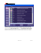
AORM Software Package SETUP AND MEASUREMENT DIALOG The “AORM Measurements” dialog is accessed from the menu bar’s Analysis menu. AORM is supplied with X-Stream software version 4.2 and later.
10 ISSUED: June 2013 923133 Rev A
AORM Software Package AORM Measurement Menus F i e ld D e scr i pt i on View Allows you to quickly select the most common views, with graphing. Measurement Selects the primary measurement to be made. In the Parameter view, the result for the selected measurement is displayed along with other parameters. Units The units used for the horizontal parameter results. Absolute refers to voltage or time units. Percent refers to results being calculated as a percent of the clock period.
F i e ld Show Data D e scr i pt i on Determines which table of values is displayed below the grid. When Parameters is selected, a checkbox is displayed that enables you to turn on or off the display of statistics values. Source This can be a channel, math function, or memory trace. A Use Equalizer checkbox is provided to apply a filter to the data source. Data Gate This can be a channel, math function, memory trace, or other.
AORM Software Package F i e ld D e scr i pt i on The clock need only be specified if the parameter requires a clock for the calculation, or it is used as the source of the period. Clock/Period By selecting From Data, you can have the clock recovered from the data. In this case, all other clock setup fields except Clock Slope are unavailable. When From Clock is selected, the period is automatically measured from the clock provided. The clock must then be configured.
F i e ld Subject nT Preceded by low nT Preceded by high nT From nT To nT 14 D e scr i pt i on For BES, EES, BEES, BESS, and EESS, this specifies the pit of interest. The results will be computed for each space/pit (pit/space) pair using the subject pit and all the spaces within the range specified. Specifies the range of n indices that define the pits/spaces used in the calculation. The range of n coupled with T are used to categorize the pits/spaces based on their widths.
AORM Software Package Measurement Table When the Parameter view is selected, up to 4 additional parameters, which are related to the selected measurement, are displayed. The following table shows these additional parameters. For parameters that can be shown in the XY display, it also shows the parameter that is used for the X axis.
View Menu Selections View Parameter Histogram Trend XY Plot Displays Additional Keys The source traces will be displayed along with the custom parameters (see Measurement Table, next). If two traces are to be displayed, dual grids will be drawn. Statistics: toggles the parameter statistics on/off. When Histogram is selected, a histogram of the selected parameter is displayed in a second grid, and a new tab, “AORM Histogram,” appears.
AORM Software Package Equalizer and PLL Dialog F i e ld D e sc r ipt i on T ra ck C lo ck Check this checkbox to enable tracking. Filter Cutoff and Boost An equalizer filter is applied prior to the measurements. You can adjust the cutoff frequency and boost of the filter. Slicer Bandwidth The data passes through a slicer to level the data (removes the threshold due to low frequency effects). You can set the bandwidth of the slicer.
CREATING AND ANALYZING HISTOGRAMS Selecting the Histogram Function Histograms are created by graphing a series of waveform parameter measurements. The first step is to define the waveform parameter to be histogrammed. The next figure shows a screen display accompanying the selection of a frequency (freq) parameter measurement for a sine wave on Channel 1. Four waveform cycles are shown, which will provide four freq parameter values for each histogram on each sweep.
AORM Software Package The current horizontal per division setting for the histogram. The unit type used is determined by the waveform parameter type that the histogram is based on. The vertical scale. • Linear makes the vertical scale linear. The baseline of the histogram designates a bin value of 0. As the bin counts increase beyond that which can be displayed on screen using the current vertical scale, this scale is automatically increased in a 1-2-5 sequence.
DISPLAYING TRENDS The Trend function for processing waveforms creates a graph of successive waveform parameter values. It provides useful visual information on waveform parameter variation. Used together with other scope features, it allows you to graph certain parameters compared to others. To Configure a Trend: 1. From the menu bar select Math, then Math Setup… from the drop-down menu. 2. Touch an Fx tab that is not currently assigned a math function (i.e., Zoom function by default). 3.
AORM Software Package from the Select Math 4. Touch inside the Operator1 field and select Trend Operator pop-up menu. The "Trend" setup dialog will appear at the right of the screen: 5. Decide whether all the parameter values, all per trace, or only the average of all parameter calculations for each waveform acquisition should be placed in the trend. All -- every parameter calculation on each waveform will be placed in the trend.
Trend Calculation Once the trend has been configured, parameter values will be calculated and trended on each subsequent acquisition. Immediately following an acquisition, its trend values will be calculated. The resulting trend is a waveform of data points that can be used the same way as any other waveform. Parameters can be calculated on it, and it can be zoomed, serve as the x or y trace in an XY plot, and can be used in cursor measurements. The sequence for acquiring trend data is: 1. trigger 2.
AORM Software Package • Vertical value at point in trend at cursor location when using cursors • Number of events in trend that are within unzoomed horizontal display range. • Percentage of values lying beyond the unzoomed vertical range when not in cursor measurement mode.
MAKING OPTICAL DATA MEASUREMENTS View Modes The two modes available for Optical Recording Measurements, “Custom” and “List by nT,” both display measurements either as waveform parameters or as a list of values. This chapter further describes these modes. The following table indicates which measurements can be made in each mode.
AORM Software Package Configuration Options All configuration options are available for each parameter, except as noted in this table: Dp2c x Dp2cs x BEES Subject nT Range of nT Parameter x BES x x BESS x x EES x x EESS x x EDGSH x PAA x Pit asym x Pit base x Pit max x Pit middle x Pit minimum x Pit moda x Pit num x Pit res* x Pit top x Pit width x T@pit* x Timj x * Available from Measure dialog 923133 Rev A ISSUED: June 2013 25
Configuration Menus The menus described on the following pages show how to configure any parameter. Display the AORM dialog by touching Analysis in the menu bar at the top of the screen and selecting AORM Measurements… from the drop-down menu. Touch inside the View field and select a graph display from the pop-up menu. Touch inside the Show field and select a display mode. A default group of parameters is automatically displayed when Parameter is selected.
AORM Software Package Touch inside the Measurement field and select a measurement from the pop-up menu.
Setting Levels To identify pits or spaces, thresholds and hysteresis are set. Touch inside the Data Source field and select a signal source. Check Use Equalizer to apply a filter to the Data Source. To set up the equalizer, touch the Equalizer and PLL tab. Touch inside the Data Slope field and select an edge from the pop-up menu.
AORM Software Package Touch inside the Data Gate field and select a signal source. You can also select None. Data Gate specifies the input that will be used to determine where to perform measurements on the input signal. If a Data Gate is selected, the level is assumed to be high. The Hysteresis selection imposes a limit above and below the Threshold, which precludes measurements of noise or other perturbations within this band. The width of the band is specified in divisions.
Select a clock period by having the period calculated from the clock source, by choosing a standard, or by manually setting a clock period. If you choose a clock period from a standard, you can also set a multiplier: Setting nT For BES, EES, BEES, BESS, and EESS, this specifies the pit of interest. The results will be computed for each space/pit (pit/space) pair using the subject pit and all the spaces within the range specified.
AORM Software Package Pit or Space Identification This is determined uniquely by the threshold, hysteresis, and edge polarity of threshold crossings. A positive threshold crossing indicates the start of a positive polarity pit and the end of a negative polarity space. A positive threshold crossing followed by a negative threshold crossing fully delineates a pit. A negative crossing followed by a positive crossing fully delineates a space, as illustrated in the following figure.
The hysteresis band shown in the next figure is centered on the user- selected voltage level threshold. End of space. Space fully identified Pit meets condition of crossing into Zone 3 Zone 3 Voltage Threshold Start of pit Zone 2 Pit Width Zone 1 First feature will be a pit End of pit. Start of space Pit fully identified Space meets condition of crossing into Zone 1 The hysteresis band divides the display into three zones.
AORM Software Package • For the entire signal, only a space can be identified after a pit, and only a pit can be identified after a space. • All subsequent features are identified by crossing into the appropriate zone after the end of the previous feature. For a pit this is Zone 3, and for a space it is Zone 1. The end of the previous feature is the beginning of the current feature being identified.
BES BEGINNING EDGE SHIFT Description BES provides a measurement of the time between the beginning edge of the subject n in a specified space/pit pair and the nearest specified clock edge. The measurement is calculated between the points where the data and clock signals cross selected voltage thresholds. The clock period T can be entered by the user, or measured from a user supplied clock signal, as described below.
AORM Software Package threshold Data Signal 4T 3T Clock Signal beginning edge shift Beginning Edge Shift measurement of subject 4Tpit Data Signal Clock Signal T+ t- Zoom of Positive Polarity Pit Edge -- example measurement 923133 Rev A ISSUED: June 2013 35
The measurement has configurable units. If absolute time is specified, the value is simply the time indicated above.
AORM Software Package BESS BEGINNING EDGE SHIFT SIGMA Description BESS provides a measurement of the mean, normalized standard deviation of the Beginning Edge Shift measurements (see BES).
Display Options ORM parameter calculations can be displayed, histogrammed and trended in a variety of ways. DISPLAY TYPE VALUE DISPLAYED Parameter Statistics Off Single value of the standard deviation of the mean normalized beginning edge shift values for pits/spaces of interest for last acquisition. Parameter Statistics On Average, minimum, maximum, and sigma of the beginning edge shift sigma value calculated per acquisition for all acquisitions since the last CLEAR SWEEPS operation.
AORM Software Package EES ENDING EDGE SHIFT Description EES provides a measurement of the time between the ending edge of the subject n in a specified space/pit pair and the nearest specified clock edge. The measurement is calculated between the points where the data and clock signals cross selected voltage thresholds. The clock period T can be entered by the user or measured from a user supplied clock signal, as described below.
threshold 4T 3T Data Signal Clock Signal ending edge shift Ending Edge Shift measurement of subject 4T pit Data Signal Clock Signal T+ t- Zoom of Positive Polarity Pit Ending Edge -- example 40 ISSUED: June 2013 923133 Rev A
AORM Software Package The measurement has configurable units. If absolute time is specified, the value is simply the time as indicated above.
EESS ENDING EDGE SHIFT SIGMA Description EESS provides a measurement of the mean, normalized standard deviation of the Ending Edge Shift measurements (see EES).
AORM Software Package Display Options ORM parameter calculations can be displayed, histogrammed and trended in a variety of ways. DISPLAY TYPE VALUE DISPLAYED Parameter Statistics Off Single value of the standard deviation of the mean normalized ending edge shift values for pits/spaces of interest for last acquisition. Parameter Statistics On average, minimum, maximum, and sigma of the ending edge shift sigma value calculated per acquisition for all acquisitions since the last CLEAR SWEEPS operation.
BEES BEGINNING ENDING EDGE SHIFT Description BEES provides a measurement of both the beginning and ending edge shift for a subject n pit (space) preceded and followed by a specified space (pit). (See BES and EES.) The measurement is calculated between the points where the data and clock signals cross selected voltage thresholds. The clock period T can be entered by the user, or measured from a user supplied clock signal, as described below.
AORM Software Package The next figure demonstrates the measurement of the beginning edge shift on a single subject 4T pit preceded and followed by a 3T space. In this example, the clock is specified as the positive edge. The beginning edge shift is calculated as the time difference between the beginning pit edge and the clock edge while the ending edge shift is calculated as the time difference between the ending pit edge and the clock edge.
Display Options ORM parameter calculations can be displayed, histogrammed, and trended in a variety of ways. DISPLAY TYPE VALUE DISPLAYED Parameter Statistics Off Single value of the average time between the edges of the subject n pit (space) and nearest clock edges for all subject pits (spaces) that are preceded and followed by the specified space (pits) for the last acquisition.
AORM Software Package DP2C DELTA PIT TO CLOCK Description Dp2c provides a measurement of the time between the leading edge of the pit (or spaces of interest) and the nearest specified clock edge. The measurement is calculated between the points where the data and clock signals cross selected voltage thresholds. The value calculated depends on the clock and data edges selected, as shown in the table below.
Data Signal Clock Signal Delta Pit-to-Clock measurement Data Signal Clock Signal tn , t+ Tn, T+ tTZoom of Positive Polarity Pit Edge - example measurement 48 ISSUED: June 2013 923133 Rev A
AORM Software Package The measurement has configurable units. If absolute time is specified, the value is simply the time as indicated above. If percent is specified, the value of the measurement is the time normalized to the local clock period.
DP2CS DELTA PIT TO CLOCK SIGMA Description Dp2cs provides a measurement of the mean, normalized standard deviation of the Delta Pit-toClock measurements (see Dp2c).
AORM Software Package Display Options ORM parameter calculations can be displayed, histogrammed, and trended in a variety of ways. DISPLAY TYPE VALUE DISPLAYED Parameter Statistics Off Single value of the standard deviation of the mean normalized Delta Pit-to-Clock values for pits/spaces of interest for last acquisition. Parameter Statistics On Average, minimum, maximum and sigma of the Delta Pit-to-Clock sigma value calculated per acquisition for all acquisitions since the last CLEAR SWEEPS operation.
EDGSH EDGE SHIFT Description Edge Shift provides a measurement of the difference between the width of pits, spaces, or both, and their ideal widths. These ideal widths are integer multiples of the clock period ‘T’. The width of the pit or space is determined by the time between crossings of the selected voltage threshold (see pwid).
AORM Software Package DISPLAY TYPE VALUE DISPLAYED Parameter Statistics Off All values of the overall edge shift for all pits/spaces within the selected ‘nT’ range for last acquisition. Parameter Statistics On Average, minimum, maximum, and sigma of all edge shift values calculated per acquisition for all acquisitions since the last CLEAR SWEEPS operation. nT Table List of values of the overall edge shift for each group of pits/spaces of common ‘nT’ width for the last acquisition.
More On Edge Shift A good approach to understanding the operation of the edge shift parameter with different modes of operation starts by considering the next figure, a histogram of 3T to 5T pit widths. voltage threshold 1.16 µs 5T 690 ns 695 ns 3T 3T 920 ns 4T Histogram of Pit Widths Population 600 400 200 0 2.5 3 3.5 4 4.5 5 Pit Width / T 3T Widths 4T Widths 5T Widths The Edge Shift parameter takes on each of these distributions separately.
AORM Software Package Histogram of Edge Shifts 800 Population 600 400 200 0 30 20 10 0 10 20 30 Edge Shift in Percent 3T Edge Shift 4T Edge Shift 5T Edge Shift Superposition of Edge Shift Distributions The 3T, 4T, and 5T distributions are obtained when the Edge Shift custom parameter is configured for single n values and histogrammed.
PAA PIT AVERAGE AMPLITUDE Description Pit Average Amplitude provides a measurement of the average amplitude of pits and spaces. The calculation is performed by calculating the difference between the average value of the base (pbase) for spaces of a particular ‘nT’ width and the average value of the top (ptop) of pits of the same ‘nT’ width. For example, the average value of the base for all 3T spaces is subtracted from the average value of the top for all 3T pits to obtain the 3T pit average amplitude.
AORM Software Package Example Consider this persistence plot of an optical data waveform. Using cursors, the average amplitude of the 3T pits/spaces can be estimated. In this case, the value obtained is 47.2 mV. When the parameter paa is configured for 3T widths, the measurement result is also 47.2 mV. This value is calculated automatically.
PASYM PIT ASYMMETRY Description Pit Asymmetry provides a measurement of the asymmetry of the middle voltage level for the high nT index pits/spaces compared to the middle voltage level of the low ‘nT’ index pits/spaces. The measurement calculation is compliant with the definition of Pit Asymmetry as defined by IEC 908:1987 Section 3.1. The negative value of the measurement is referred to as Pit Symmetry as defined by ISO/IEC 10149:1995 (E) Section 12.2.
AORM Software Package Example This persistence plot of a bandwidth limited, smooth waveform illustrates asymmetry. Notice that the midlevel of the 3T waveform is offset from 0 V, and that the midlevel of the 11T waveform is approximately 0 V. Since the 3T middle level is offset, the expected asymmetry value is negative. This is the asymmetry calculated from a waveform with several thousand widths. The values are the asymmetry, the 3T middle level, the 11T middle level, and the 11T average amplitude.
PBASE PIT BASE Description Pit Base provides a best estimate of the bottom amplitude of a space. The concept of the base calculation is to automatically provide the same measurement that would be obtained from a persistence plot. The base of each space is determined through histogramming techniques described under Base and Top Calculation Details. When pbase is configured as a custom parameter, all bases within the single nT or range of nT are calculated.
AORM Software Package Example This persistence waveform is created by setting a SMART Trigger® to capture only 4T spaces. The 4T base computed is -27.0 mV. When the same measurement is taken with the parameter cursors, it confirms that -27.0 mV is a reasonable value for the base.
PMAX PIT MAXIMUM Description Pit Maximum provides a measurement of the maximum voltage value of pits of interest. It provides a comparison of how the maximum point in the waveform corresponds to the ptop value When pmax is configured as a custom parameter, all maximums within the single nT or range of nT are calculated. Histogramming or trending such a configuration would result in one value per pit in the nT range contributing a value to the histogram or trend.
AORM Software Package Example: This waveform contains a single pit, whose max is computed as 26.1 mV. The same measurement is verified using the measurement cursors.
PMIDL PIT MIDDLE LEVEL Description Pit Middle Level provides a measurement of the middle voltage level of pits or spaces. It is performed by first calculating the midpoint of the average value of the base (pbase) for spaces and the average value of the top of pits (ptop). If only 3T pits are specified, the resulting measurement is the ‘decision level’ (see ISO/IEC 10149:1995 (E) Section 12.1).
AORM Software Package Example This waveform contains thousands of pits. In ‘nT Table’ mode, the middle levels are displayed for each nT index. These values are the midlevels of the tops and bases for pits/spaces within the nT indices. The overall middle level is calculated based on a weighted average of the middle level for each nT. This value is the overall best threshold value for all pits/spaces within the 3T to 11T range.
PMIN PIT MINIMUM Description Pit Minimum provides a measurement of the minimum voltage value of pits of interest, and a comparison of how the minimum point in the waveform corresponds to the ptop value. When pmin is configured as a custom parameter, all minimums within the single nT or range of nT are calculated. Histogramming or trending such a configuration would result in one value per pit in the nT range contributing a value to the histogram or trend.
AORM Software Package Example This waveform contains a single space. The pit min is computed as -9.7 mV. The measurement can be verified with the measurement cursors.
PMODA PIT MODULATION AMPLITUDE Description Pit Modulation Amplitude provides a measurement of the ratio of the Pit Average Amplitude (paa) for the low ‘nT’ pits/spaces in the data signal to the Pit Top (ptop) of the high ‘nT’ pits in the data signal: PMODA = paalow _ n avg (top) high _ n The low and high ‘nT’ values to be used for performing the calculation are provided by the user through the associated measurement configuration options.
AORM Software Package Example The following persistence plots were generated using the DC-coupled signal. In the first plot, the amplitude measurement cursor is reading the 11T top voltage of 76.
In the second, the cursor reads the difference between the 11T top and base of 67.2 mV. In the third plot, the cursor reads the difference between the 3T top and base of 47.2 mV.
AORM Software Package The last plot shows the waveform with the parameters calculated automatically. 1. pmoda 3T paa/11T top 2. pmoda 11T paa/11T top 3. paa 3T 4. paa 11T 5. top 11T P1 contains the ratio of P3 to P5. P2 contains the ratio of P4 to P5.
PNUM PIT NUMBER Description Pit Number provides a measurement of the number of pits or spaces of interest or both. When pnum is selected as a parameter measurement the total number of pits and/or spaces for the selected ‘nT’ range is displayed. In the nT Table mode the number for each ‘nT’ value is displayed. Display Options ORM parameter calculations can be displayed, histogrammed, and trended in a variety of ways.
AORM Software Package Example In this waveform, each of the 3 pits/spaces is easily identified. There is a 4T pit, a 6T space, and a 5T pit. Each is counted and displayed in ‘nT Table’ mode. This is the long waveform showing the number of pits/spaces obtained: approximately 9,000.
PRES PIT RESOLUTION Description Pit Resolution measures the ratio of the Pit Average Amplitude (see paa measurement description) of the smallest of the ‘nT’ pits or spaces in the data signal to that of the largest: PRES = paalow _ n paahigh _ n ⋅ 100% The low and high ‘nT’ values for performing the calculation must be provided by the user through the associated measurement configuration options. The value shown is in units of percent.
AORM Software Package Example Consider the following persistence plots. In the first, the amplitude measurement cursor reads the difference between the 3T top and base: 47.3 mV. In the second, the cursor reads the difference between the 11T top and base: 67.3 mV.
This is the same waveform with the parameters calculated automatically. 1. pres 3T paa / 11T paa 2. paa 3T 3. paa 11T P1 contains the ratio of P2 to P3 in percent.
AORM Software Package PTOP PIT TOP Description Pit Top provides a measurement of the best estimate of the top amplitude of a pit. The concept of the top calculation is to automatically provide the same measurement which would be obtained from a persistence plot. The top of each pit is determined through histogramming techniques described in detail under Base and Top Calculation Details. When ptop is configured as a custom parameter, all tops within the single nT or range of nT are calculated.
Example This persistence waveform was created by setting a SMART Trigger to capture only 3T pits. The computed 3T top is 25.8 mV. When the same measurement is taken with the parameter cursors, it confirms that 25.8 mV is a reasonable value for the top.
AORM Software Package PWID PIT WIDTH Description Pit Width provides a measurement of the width of pits or spaces or both. The width of the pit or space is determined by the crossing of the selected voltage threshold. When pwid is selected as a parameter measurement it is generally useful to display the measurement calculation for a single ‘nT’ value. Otherwise the measurement will calculate the average width of 3T pits, 4T pits, and so on, which is meaningless.
Example The example shows that, measured at the selected voltage threshold, the CD data signal contains sequentially a 5T pit, 3T space, 3T pit, and 4T space. If the measurement is configured to select only 3T pits or spaces then the value displayed will be: pwid = (694 ns + 696 ns) / 2 = 695 ns voltage threshold 5T 1.16 µs 3T 694 ns 3T 696 ns 4T 925 ns Example 2: Histogramming Consider the problem of determining the error margin in an optical recording system.
AORM Software Package 1. Use the maximum number of values (2,000,000,000) 2. Classify into 2000 bins 3. Linear vertical scale. The trigger is set up to trigger on a pit edge and operated in normal trigger mode. Note: Prior to acquisition, select each trace and press the RESET button to ensure that all the traces are reset. In normal trigger mode, multiple waveforms are acquired and processed. The histogram will typically have data that is not well centered or is off screen.
By enabling cursor tracking, the difference cursors are swept across the histogram. As expected, the space between the 3T and 4T distributions is the shortest, because of inter-symbol interference and the many 3T widths. The spacing is 138 ns. To measure the spread of widths for the distributions, set the measure mode to My Measure and configure the parameters: 1. P2: average of F2 2. P3: high of F2 3. P4: low of F2 4.
AORM Software Package This screen shows the histogram statistics taken on the 5T distribution. The distribution has the largest spread of values: 102.5 ns. The mean is 1.1659 µs, which is 3.6% higher than the ideal of 1.1575 µs.
T@PIT TIME AT PIT Description The Time-at-Pit parameter provides the time of each leading edge of every pit or space within the nT range specified from the trigger point (time = 0). The value displayed is the time of the first pit only. The usefulness of this parameter is not in the displayed value, but in its trending.
AORM Software Package We are expecting 1800 p its/spaces, so make sure that the trends are set to use up to 2000 values for each math setup. The trigger is set up to trigger on a pit edge and is operated in single-shot mode. For convenience, the waveforms are ordered on the screen in a particular manner: 1. F2: Trend of t@pit 2. F1: Trend of pwid 3. F3: Zoom of optical recording waveform The reason for this order will become apparent. Press the single-shot trigger button to acquire the waveform.
The waveforms are displayed in Quad grid mode. The trend of t@pit is basically linear, as expected because the time at each pit from the trigger is ascending. The trend of the pit widths looks basically as expected. Notice that there are exactly as many events inside both trends, a necessary condition. From the menu bar, select Display Setup… and set the grid mode to XY. Bands of pit widths corresponding to widths that are ideal integer multiples of the clock period will be evident.
AORM Software Package The XY plot has been adjusted so that all the pit widths are displayed vs. time. Notice that all form bands. This is because all but two are ideal integer multiples of the clock period. The two pit widths dissimilar to the others are sitting just below the 3T pit width band, and between the 4T and the 5T band. These strange pit widths occurred around the middle of the waveform.
waveform so that the cursor on the trace is at the center of the screen. Expand the waveform using the horizontal zoom control. Here is the waveform zoomed in a bit with the measurement cursor placed at 859.600 µs. As can be seen, there is some kind of aberration at the center of the trace.
AORM Software Package Further zooming clearly identifies the problem: a burst error that prevented the positive polarity width that starts at 859.61 µs from reaching its peak value. This defect caused the reflectivity to drop and to erratically fluctuate throughout the duration of the burst error. The defect affected the width of the next pit as well, which created the pit width centered between the 4T and 5T band of the XY plot.
TIMJ TIMING JITTER Description Timing Jitter provides a measurement of the standard deviation of the difference of the width of pits and/or spaces from the mean width. The width of the pit/space is determined by the crossing of the selected voltage threshold. The measurement calculation is compliant with the definition of Timing Jitter as defined by ISO/IEC JTC1.23.14517 Section 22.4. Display Options ORM parameter calculations can be displayed, histogrammed, and trended in a variety of ways.
AORM Software Package The 3T timing jitter is calculated by taking the standard deviation of the difference between each width and the 3T mean. This is 3.214 ns, normalized by: Timj3T = 3.214 ⋅ 100% = 1389% . 2315 . The 4T timing jitter cannot be calculated because there is only one value (at least two values are required). The 5T timing jitter is +6.109%. The overall timing jitter is calculated using a weighting formula, which results in the standard deviation of the mean centered distributions.
More About Timing Jitter In order to understand the operation of the timing jitter parameter with different modes of operation, consider the histogram of 3T to 5T pit widths in the next figure. Histogram of Pit Widths Population 600 400 200 0 2.5 3 3.5 4 4.5 5 5.5 Pit Width / T 3T Widths 4T Widths 5T Widths The Timing Jitter parameter considers each of these distributions separately. For each distribution the standard deviation is calculated.
AORM Software Package Mean Normalized Width Distributions 800 Population 600 400 200 0 30 20 10 0 10 20 30 Mean Normalized Width (%) 3T Mean Normalized Widths 4T Mean Normalized Widths 5T Mean Normalized Widths Resulting Superposition The value displayed on the custom parameter line (with statistics off) is the sigma of any of the resulting distributions for the last acquisition only. This timing jitter value is calculated internally without having to actually histogram the values.
SIGNALS, COUPLING, AND THRESHOLD SETTINGS Which optical recording signal, or combination of signals should be used in a calculation? How should the signal be coupled, or the threshold set? The answers to these questions are sometimes uncertain. This appendix offers tips on how to answer them. Choice of Signals Generally, the choice of signals depends on the aim of the measurement.
AORM Software Package In the case of threshold-insensitive parameters, it usually suffices to use a fixed threshold somewhere in the middle of the optical recognition waveform. Even if the signal’s middle shifts, the fixed threshold is usually adequate. Additionally, if the signal is AC coupled, it will tend not to shift much, and the fixed threshold will be perfectly adequate. The problem arises when what is required is a DC-coupled signal with a threshold that changes dynamically throughout the waveform.
USING PARAMETERS WITH TRENDS AND XY PLOTS X-axis Y-axis t@pit Dp2c edgsh pbase pmax pmin ptop pwid pwid We saw in the t@pit parameter description how the ORM parameters have certain unique characteristics that make particular measurements useful when trended together with XY plots. And how the t@pit parameter is essential to those measurements. Plots that can be generated on single acquisitions include those listed in the table at left.
AORM Software Package The trigger is set to trigger on a pit edge and is operated initially in single-shot mode. For convenience, the waveforms are ordered on the screen in a particular manner so that they will automatically work correctly with XY display mode: 1. F2: Trend of t@pit 2. F1: Trend of pwid 3. Channel 1: optical recognition data signal Note: Prior to acquisition, select each trace and press the RESET button to ensure that all the traces are reset.
This is what the XY plot looks like: The XY plot has been adjusted so that all of the pit tops are displayed vs. Pit width. Notice that all of the pit widths form clusters. Press NORMAL trigger, and the clusters will become even more dense. You can have up to 20,000 points in the XY plot. Using the XY cursors, a variety of measurements can be performed simultaneously. For example, here it can be seen that the 5T pit width varies by approximately 82 ns and the top varies by approximately 2.58 mV.
AORM Software Package IMPROVING HORIZONTAL MEASUREMENT ACCURACY Horizontal measurement accuracy pertains to timing-related measurements. In the AORM package, these are Dp2c, Dp2cs, edgsh, lper, pwid, t@pit, and timj. In many cases, measurement accuracy can be improved by considering certain items pertaining to how a DSO operates and how parameters are measured. DSOs sample the signal, building a waveform that consists of points at intervals determined by the sample rate.
BASE AND TOP CALCULATION DETAILS The base and top are designed to emulate results in the past obtained from persistence plots. In general, the top was calculated by examining the most intense region near the top of a waveform in an eye-pattern persistence map. The AORM package improves on this in that the tops of all pits are calculated independently: rogue amplitude variations in the waveform can be identified. The waveform in the next figure contains two pits. We need only consider the first of these.
AORM Software Package The AORM package histograms the values inside each pit to determine the most likely amplitude: the most densely populated region. The next figure shows the histogram of the pits’ amplitudes. It is easily seen that the most likely amplitude is approximately 32 mV (exactly 31.9 mV). The top is calculated by averaging all of the waveform data points at or above this, to give a result of 32.89 mV. Histogram of Waveform Points Population 150 100 50 0 0 0.005 0.01 0.015 0.02 0.
Top Calculation 0.04 Amplitude (mV) 0.035 0.03 0.025 0.
AORM Software Package THEORY OF OPERATION An understanding of statistical variations in parameter values is needed for many waveform parameter measurements. Knowledge of the average, minimum, maximum, and standard deviation of the parameter may often be enough, but in many other instances a more detailed understanding of the distribution of a parameter’s values is desired. Histograms provide the ability to see how a parameter’s values are distributed over many measurements.
Count 40 30 20 10 1.5 2 3 3.15 Range 4 4.35 5 6 Volts The sequence for acquiring histogram data is: 1. trigger 2. waveform acquisition 3. parameter calculations 4. histogram update 5. trigger re-arm. If the timebase is set in non-segmented mode, a single acquisition occurs prior to parameter calculations. However, in Sequence mode an acquisition for each segment occurs prior to parameter calculations.
AORM Software Package Histogram Parameters Once a histogram is defined and generated, measurements can be performed on the histogram itself. Typical of these are the histogram’s: • Average value, standard deviation • Most common value (parameter value of highest count bin) • Leftmost bin position (representing the lowest measured waveform parameter value) • Rightmost bin (representing the highest measured waveform parameter value). Histogram parameters are provided to enable these measurements.
maxp population of most populated bin in histogram mode data value of most populated bin in histogram pctl data value in histogram for which specified ‘x’% of population is smaller pks number of peaks in histogram range difference between highest and lowest data values sigma standard deviation of the data values in histogram totp total population in histogram xapk x-axis position of specified largest peak.
AORM Software Package Determining such peaks is very useful because they indicate the dominant values in a signal. However, signal noise and the use of a high number of bins relative to the number of parameter values acquired can give a jagged and spiky histogram, making meaningful peaks hard to distinguish. The scope analyzes histogram data to distinguish peaks from background noise and from histogram definition artifacts such as small gaps, which are due to very narrow bins.
DVD PROCESSING MODEL In many applications, it is important to make measurements directly from the RF signal, independent of a specific DVD chip. The OData processing function provided in the Advanced ORM package can emulate the filter, slicer, and/or phase-locked loop (PLL) of a typical optical recording drive. A schematic of this function is shown in the following diagram. You can view the equalized, leveled data, threshold, sliced data, or the extracted clock.
AORM Software Package Equalized Leveled Slicer RF data Filter Σ Sliced Threshold fc, boost bandwidth PLL User input Extracted Clock bandwidth Where: • Equalized – applies a low pass filter with boost to the input data. This should not be used if the input data is already equalized (filtered). • Leveled – Applies the filter (if the input data is raw RF) and then subtracts the sliced threshold from it. • Sliced – This is the output of the slicer.
FILTERING A low-pass filter that removes high-frequency noise and provides equalization is needed for the newer optical recording systems (e.g., DVD). In the DVD read-only and recordable specifications are given the frequency characteristics of the low pass filter (LPF) and equalizer (EQ) as a graph. The combination of these must meet within 1 dB below 7 MHz, and it is recommended to meet it up to 10 MHz. Also, group delay variation for frequencies /= ±3 ns, and gain at 5.
AORM Software Package Gate 923133 Rev A Optionally, you can specify a channel that will be used to gate the input signal. When specified, you must also specify the polarity of the gate (i.e., process when low or high).
APPENDIX A: NOTES ON ODATA MATH FUNCTION The ORDATA math function can accept as input either unequalized or already equalized data, and produce: • Equalized: If the input data is not already equalized, the instrument applies equalization using the Filter Cutoff and Boost settings from the "Equalizer and PLL" dialog.
AORM Software Package • "Acquisition too small to apply EQ filters": The valid region of the waveform is reduced by "EQ spacing" (see following explanation) on each side. This error message means that the result would then have no valid points. • "LP fc low & sample rate too high, can't EQ filter": This message is shown if current EQ spacing is greater than 8191 samples, an implementation restriction.
4 4 5 .10 6 3.2 2.9 3 2 1 20 .log Spec k Re Spec k 0 Im Spec k 1 2 3 4 4 0 0 2 10 6 6 4 10 6 6 10 spec_f( k ) 8 10 6 7 1 10 7 1.2 10 6 12 .10 Simulation result showing transfer function of the digital low-pass filter and 3-tap EQ (boost) filter, set to 8.2 MHz cutoff frequency and 3.2 dB boost. Leveled There are no additional conditions to produce leveled data. The threshold is calculated and subtracted even if the equalization could not be applied for the reasons described above.
AORM Software Package trace; and it can be used for measurements of the clock frequency. If the JTA option is present, a JitterTrack of Frequency of the extracted clock may give interesting insight into timing variation in the input signal. The only user-set parameter for clock extraction is the "PLL BW" setting on the "Equalizer and PLL” dialog. The PLL Bandwidth is the unity gain intercept of the open-loop transfer function of the PLL. The closed loop -3 dB frequency is approximately 1.274 time that.
Since the acquired data may be a millisecond or less in duration, extracting the clock depends critically on the scope’s ability to determine T (1/clock frequency) from the data and on starting the PLL's VCO at that frequency and at about the right phase. When it can do that, the VCO starts up locked and does not have to settle noticeably. If it cannot find the frequency, the warning message: "ORDATA VCO start freq is 3.19*LP fc, didn't find it” will be displayed.
AORM Software Package A small section of a 1 ms long noisy DVD waveform. Acquired with an ungrounded AP020 probe at 500 MS/s.
Same piece of the same signal, equalized and leveled.
AORM Software Package It should be mentioned that the extracted clock output is also exactly five divisions high (without vertical zoom), and its edges are linear from -0.1 to +0.1 * T and from +0.4 to +0.6 * T. Therefore, if there are 20 samples per T, each edge of the extracted clock signal has four samples between the top and base. These samples are placed proportional to phase, so that the edge crosses 0 at exactly 0 and 180 degrees VCO phase.
Roughly, the phase steering target for the VCO is that the data transitions should happen on the falling edge of the VCO output. To be more precise, we steer such that the VCO phase will be 180 degrees at the sample where a zero crossing in the data is detected. Because the software VCO works on a sample-by-sample basis, there is, on average, a half-sample delay from the VCO falling edge's zero cross to the data zero cross. At 20 samples per T, this half-sample error is 2.
AORM Software Package edges. If the source waveform has less than 2000 edges, the accuracy of this procedure may be reduced. If the source waveform has less than 50 edges, the instrument does not even attempt to estimate T. The PLL will start at 3.19024 * LP fc. Because of the low bandwidth of the PLL, it does not make much sense to try to extract the clock from a very short waveform; the PLL will not have time to react.
the frequency is disturbed slightly for the first 15 µs or so; the frequency shift during this time is very small, on the order of 0.1%, as the phase adjusts.