QPHY-SAS2 SAS2 Serial Data Operator’s Manual Revision A – March, 2010 Relating to the Following Release Versions: Software Option Rev. 6.1 SAS2 Script Rev. 1.0 Style Sheet Rev. 1.
LeCroy Corporation 700 Chestnut Ridge Road Chestnut Ridge, NY, 10977-6499 Tel: (845) 578-6020, Fax: (845) 578 5985 Internet: www.lecroy.com © 2009 by LeCroy Corporation. All rights reserved. LeCroy and other product or brand names are trademarks or requested trademarks of their respective holders. Information in this publication supersedes all earlier versions. Specifications are subject to change without notice.
QPHY-SAS2 Software Option TABLE OF CONTENTS INTRODUCTION ........................................................................................................................ 6 Compatibility ............................................................................................................................................................... 6 SETUP AND INSTALLATION ................................................................................................... 6 Required Equipment ...........
Cable Deskewing using the Fast Edge Output (WavePro 7 Zi and WaveMaster 8Zi only) ..................................... 40 Cable Deskewing without using the Fast Edge Output ............................................................................................ 43 File name conventions for saved waveform data .....................................................................................................
QPHY-SAS2 Software Option FIGURES Figure 1 - Report menu in QualiPHY General Setup............................................................................................. 7 Figure 2 - The Test Report includes a summary table with links to the detailed test results .......................... 8 Figure 3 - QualiPHY main menu and compliance test Standard selection menu ............................................ 10 Figure 4 - QualiPHY configuration selection menu .........................................
INTRODUCTION QPHY-SAS2 is a software package designed to capture, analyze, and report measurements in conformance with UNH IOL Serial Attached SCSI (SAS) Consortium SAS-2 6Gbps Physical Layer Test Suite (Version 1.01). A copy of the specification can be found on the UNH IOL FTP site. Note: As of March 2nd, 2010 this document can be found at the following site but this is subject to change: ftp://ftp.iol.unh.edu/pub/sas/test_suite/SAS-2_6Gbps_Physical_Layer_Test_Suite_(v1.01).pdf.
QPHY-SAS2 Software Option QUALIPHY COMPLIANCE TEST PLATFORM QualiPHY is LeCroy‟s unique compliance test framework which leads the user through the compliance tests. QualiPHY displays connection diagrams to ensure tests run properly, automates the oscilloscope setup, and generates full compliance reports. QualiPHY makes SAS-2 compliance testing easy and fast. The QualiPHY software application automates the test and report generation.
See the QualiPHY Operator’s Manual for more information on how to use the QualiPHY framework.
QPHY-SAS2 Software Option Oscilloscope Option Key Installation An option key must be purchased to enable the QPHY-SAS2 option. Call LeCroy Customer Support to place an order and receive the code. The software option SDA2 is also required. Enter the key and enable the purchased option as follows: 1. From the oscilloscope menu select Utilities Utilities Setup... 2. Select the Options tab and click the Add Key button. 3. Enter the Key Code using the on-screen keyboard. 4.
QualiPHY tests the oscilloscope connection after clicking the Start button. The system prompts you if there is a connection problem. QualiPHY‟s Scope Selector function can also be used to verify the connection. Please refer to the QualiPHY Operator’s Manual for explanations on how to use Scope Selector and other QualiPHY functions. Accessing the QPHY-SAS2 Software using QualiPHY This topic provides a basic overview of QualiPHY‟s capabilities.
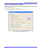
QPHY-SAS2 Software Option 4. Click the Configuration button in the QualiPHY main menu: 5. Select a configuration from the pop-up menu: Figure 4 - QualiPHY configuration selection menu 6. Click Start. 7. Follow the pop-up window prompts.
Customizing QualiPHY The predefined configurations in the Configuration screen cannot be modified. However, you can create your own test configurations by copying one of the standard test configurations and making modifications. A description of the test is also shown in the description field when selected.
QPHY-SAS2 Software Option Creating Custom Configurations Beginning with any of the pre-loaded configurations, 1. Click on the Test Selector tab to change what tests you would like to be included in your new configuration. 2. Click on the Variable Setup tab to change the variables for your new configuration. 3. Click on the Limits tab to change which limit set should be used for your new configuration See QualiPHY Manual for more information 4.
Figure 6 - Variable Setup and Limits Manager windows 14 917718 Rev A
QPHY-SAS2 Software Option USING THE LECROY SIERRA M6 FOR SAS TRANSMITTER TESTING The LeCroy Sierra M6 protocol analyzer can be used to stimulate SAS-2 targets to output the required test patterns for SAS-2 transmitter testing. Required Equipment LeCroy Sierra M6-4 or M6-2 SAS Protocol Analyzer LeCroy Protocol Suite Utility is required to control the Sierra This is available from www.lecroy.com.
Procedure 1. Be sure the SAS Protocol Suite utility supplied with the SIERRA M6 is installed. (The directories below may change depending upon your installation choices) 2. Copy the sas2 phy diagnostic page.sac file to the following directory: C:\Users\Public\Documents\LeCroy\SAS Protocol Suite\User. 3. Copy the SAS2_PortA_Diagnostics.txt and SAS2_PortB_Diagnostics.txt files to the following director: C:\Users\Public\Documents\LeCroy\SAS Protocol Suite\System\DataBlock. 4.
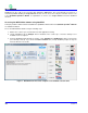
QPHY-SAS2 Software Option 7. Using the Find Device selection under the Tools menu, you will get the dialog below. Set it for T1 and click on “Find device”. Figure 9 - Device Identifier 8. This warning message appears. Select the “Yes” option. He resulting operation can take up to 30 seconds. Figure 10 - Warning Message If the search for device succeeds, the resulting dialog will look like this with the SAS Address shown in the upper left.
Figure 11 - Device Identifier with Device Address Shown 9. Record the Address shown in the Device List 10. Click on the Close button on the Device Identifier list. 11. Click on File -> Open and select the sas2 phy diagnostic page.sac file. a. This file should be shown in the default directory where the file was previously copied. b. This file contains the SCSI commands and diagnostic information you will need to control the device‟s diagnostic modes.
QPHY-SAS2 Software Option Figure 12 - LeCroy SAS Protocol Suite with SAC file loaded 12. In the Target SAS Address field, enter the address previously recorded from the Device Identifier screen. 13.
Figure 13 – LeCroy SAS Protocol Suite Data Block Configuration 14. Click on the Delete All button to delete the current data block information 15. Click on the Load button (lower right corner) to select a new data block to load. a. Select SAS2_PortA_Diagnostics.txt to load the data block for testing the A (primary) port of the target. b. Select SAS2_PortB_Diagnostics.txt to load the data block for testing the B (secondary) port of the target. 16.
QPHY-SAS2 Software Option Figure 14 – LeCroy SAS Protocol Suite Closing the Data Block Window 17. Click the Yes button to save the changes to the data block. 18. Clicking the arrow on the right side of the Payload Data field will display a list of available commands to send the target under test. 19. At power-on of the SAS-2 device, it should be in the “stopped” mode. In this mode it will be transmitting the “Out of Band” signal (common to all 3 speeds of SAS-2).
Data Block Selections A_STOP_COMINIT This is used to stop the current data output and return to OOB state. This must be sent in order to change patterns. A6G_SCR_0 Sends the 6Gbps Scrambled Zero Pattern A6G_HFTP Sends the 6Gbps HFTP Pattern A6G_MFTP Sends the 6Gbps MFTP Pattern A6G_Idle Sends the 6Gbps Electrical Idle Pattern A6G_D30p3 Sends the 6Gbps D30.
QPHY-SAS2 Software Option QPHY-SAS2 OPERATION After pressing Start in the QualiPHY menu, the software instructs how to set up the test using pop-up connection diagrams and dialog boxes. QualiPHY also instructs how to properly configure the Product Under Test (PUT) to change test signal modes (when necessary).
QPHY-SAS2 TEST CONFIGURATIONS Configurations include variable settings and limit sets as well, not just test selections. See the QPHY-SAS2 Variables section for a description of each variable value and its default value. 1.5 Gbps Tx tests using Live (Acquisition) Data This configuration will run all of the tests except for the deskew tests and the WDP test. The limit set in use is SAS2-1.5G. All of the variables are set to their default settings except Bitrate is set to 1.5e9. 1.
QPHY-SAS2 Software Option QPHY-SAS2 VARIABLES Use the Upper (A) or Lower (B) Input For oscilloscope with 2 inputs per channel (Zi series oscilloscope >= 4 GHz bandwidth), this variable allows the user to decide whether to use the A or B input to run the selected tests. The default value for this variable is InputA. Bitrate for SAS2 This variable allows the user to specify the bitrate that is being used for testing. The default value for this variable is 6e9.
Tx Positive Source The variable allows the user to select the input source used for Tx postive signal. The default value for this variable is C2.
QPHY-SAS2 Software Option QPHY-SAS2 TEST DESCRIPTIONS Tx Group 1 Out of Band Tests 5.1.x (OOB) There are 4 tests run in this group. The tests that are run are: 1. 5.1.2 – Tx Maximum Noise During OOB Idle 2. 5.1.3 – Tx OOB Burst Amplitude 3. 5.1.4 – Tx OOB Offset Delta 4. 5.1.
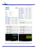
Figure 18 - OOB Test Results In the Measure section: IdleNoise (P1) is the peak-to-peak measurement of F3 (idle differential signal). This is the measured value for Tx – Max Noise During Idle (5.1.2). This value must be less than 120mV(P-P) in order to pass the test. OffsetDelta (P3) is the mean amplitude of F4 (burst differential signal). This is the measured value for Tx- OOB Offset Delta (5.1.4). This value must be between -25mV and 25mV (inclusive) in order to pass the test.
QPHY-SAS2 Software Option Figure 19 - Oscilloscope Configuration after SSC Tests Shown on this screen: th F2 is the SSCTrack of the input. This signal is filtered by a 4 order Butterworth filter with a 200kHz cutoff as described by the specification. th F3 is the SSCTrack of the input without the effects of the 4 order Butterworth filter used by F2. F4 is the Rate of Frequency Modulation (dF/dT). This is calculated by: slope = (f(t)–f(t–0.27us))/0.27 us).
MinDFDT and MaxDFDT (P9 and P10) are calculated by measuring the minimum and maximum of the DFDT (F3). This is the measured value for Tx- SSC DFDT Min and Tx- SSC DFDT Max (5.2.4). These values must be between +/-850pm/us in order to pass this test. Imbalance (P12) is measure of the deviation asymmetry of the DFDT. It is measured by taking the absolute value of the sum of the averaged max peak level and the averaged min peak level. This is the measured value of Tx – Deviation Asymmetry (5.2.3).
QPHY-SAS2 Software Option F2 is the SSCTrack of the input. This signal is filtered by a 1 order Butterworth filter with a 3.7 MHz cutoff as described by the specification. The first division of the result is discarded to allow for clock recovery “capture” as well as settling of the startup effect of the filter. This is the same as creating the SSCTrack, however, when SSC is not enabled on the device, we can use this to calculate the long term stability.
In the Measure section: CM Offset (P1) is the common mode offset. This is measured by taking the mean of the common mode trace. This is the measured value of Tx – Common Mode Offset (5.3.2). This test is informational only. CM RMS (P2) is the common mode RMS voltage. This is measured by taking the RMS of the common mode trace. This is the measured value for Tx – CM RMS voltage (5.3.2). This value must be less than 30mV in order to pass this test. Tx 5.3.4 and 5.3.5 Vpp, VMA, EQ (D30.
QPHY-SAS2 Software Option Figure 26 - Vpp, VMA and EQ Results In the Measure section: Vpp (P1) is measuring the full range of the F4 histogram. This is the measured result for Tx - Vpp (5.3.4). This value must be between 850mV and 1.2V in order to pass this test. LowMode (P4) is the maximum peak from the left side of the F5 waveform. This represents the deemphasized low voltage level of the signal. HighMode (P5) is the maximum peak from the right side of the F5.
F4 is the histogram of all of the measured 20-80 rise times. Z2 is a zoom of F1. Figure 28 - Rise and Fall Times Results In the Measure section: Rise 20-80 (P1) is 20-80 rise time of the differential input waveform (F1). Fall 80-20 (P2) is the 80-20 fall time of the differential input waveform (F1). Rise(UI) (P3) is the 20-80 rise time converted to Unit Interval. This is the measured value of TX - Trise (20-80) (5.3.6).
QPHY-SAS2 Software Option Shown on this screen: F1 is the differential input waveform. RjBUjHist is the histogram of the random and bounded uncorrelated jitter. This is the same as the full TIE histogram with the DDj removed. The RjBUjHist is an output from SDA II. Note: For more information on SDA II refer to the Understanding SDA II Jitter Calculation Methods technical brief available at the following address: http://www.lecroy.
Figure 31 - WDP Message Box At this point that user should run the SASWDP script and enter the returned value in this dialog. By entering this value, the result for the WDP test can be included in the test report provided by QualiPHY. For more information refer to the How to run the SASWDP script section of this manual.
QPHY-SAS2 Software Option F1 is the differential input waveform. This is calculated by subtracting the negative input waveform from the positive input waveform. F2 is the resampled and interpolated waveform that has exactly 16 evenly spaced samples per UI. This waveform is also averaged to reduce Rj. This is all done in accordance with the specification. This waveform is saved in the required input format for the SASWDP script. This file is saved in the D:\Waveforms\SAS2 directory on the oscilloscope.
HOW TO RUN THE SASWDP SCRIPT The SASWDP script is required for running the Waveform Distortion Penalty (5.3.9) test. This script can be obtained from the T10 organization website (http://www.t10.org/cgi-bin/ac.pl). A valid T10 login is required for downloading this download. Note: As of March 2nd, 2010 this script can be found at the following site but this is subject to change: http://www.t10.org/cgi-bin/ac.pl?t=d&f=09-015r0.zip 1.
QPHY-SAS2 Software Option 5. Enter the value for xWDP that is returned from the SASWDP screen in the dialog box described in the Tx 5.3.9 Waveform Distortion Penalty description above.
CALIBRATION PROCEDURES Cable Deskewing using the Fast Edge Output (WavePro 7 Zi and WaveMaster 8Zi only) The following procedure demonstrates how to deskew two oscilloscope channels and cables using the fast edge output, with no need for any “T” connector or adapters. This can be done once the temperature of the oscilloscope is stable. The oscilloscope must be warmed up for at least a half-hour before proceeding.
QPHY-SAS2 Software Option Figure 37 - Trigger Settings for Deskew with the Fast Edge Output Parameter Measurements: i. Set the source for P1 to CX and the measure to Delay ii. Set the source for P2 to CY and the measure to Delay iii. Set the source for P3 to M1 and the measure to Delay Figure 38 - Measurement Settings for Deskew with the Fast Edge Output 3. Set the display to Single Grid Click Display -> Single Grid 4.
Figure 40 - Save Waveform Settings for Deskew with the Fast Edge Output 11. Disconnect Channel X from the Fast Edge Output and connect Channel Y to the Fast Edge Output. 12. Press the Clear Sweeps button on the front panel to reset the averaging. 13. Allow multiple acquisitions to occur until the waveform is stable on the screen. 14. From the Channel Y menu, adjust the Deskew of Channel Y until Channel Y is directly over the M1 trace. 15. Ensure that P3 and P2 are reasonably close to the same value.
QPHY-SAS2 Software Option Cable Deskewing without using the Fast Edge Output The following procedure demonstrates how to deskew two oscilloscope channels and cables using the differential data signal, with no need for any “T” connector or adapters. This can be done once the temperature of the oscilloscope is stable. The oscilloscope must be warmed up for at least a half-hour before proceeding. This procedure should be run again if the temperature of the oscilloscope changes by more than a few degrees. 1.
Alternately, we clearly could have not inverted C3 and instead selected the Skew clock 2 tab in the P1 parameter menu and set the oscilloscope to look for negative edges on the second input (C3).
QPHY-SAS2 Software Option SSC center-spreading High Frequency Test Pattern (10101010…) with SSC up-spreading HFTP-SSC-UP_p HFTP-SSC-UP_n 500 microseconds (or 50us/div) Medium Frequency Test Pattern (11001100…) MFTP_p MFTP_n 500 microseconds (or 50us/div) Medium Frequency Test Pattern (11001100…) with SSC down-spreading MFTP-SSC-DOWN_p MFTP-SSC-DOWN_n 500 microseconds (or 50us/div) Medium Frequency Test Pattern (11001100…) with SSC center-spreading MFTP-SSC-CENTER_p MFTP-SSC-CENTER_n 500 micro