QPHY-SAS3 Operator’s Manual Revision A – May, 2014 Relating to the Following Release Versions: • Software Version Rev. 7.4 • SAS3 Script Rev. 7.4 • Style Sheet Rev. 1.
700 Chestnut Ridge Road Chestnut Ridge, NY, 10977-6499 Tel: (845) 425-2000, Fax: (845) 578 5985 teledynelecroy.com © 2014 by Teledyne LeCroy. All rights reserved. Teledyne LeCroy and other product or brand names are trademarks or requested trademarks of their respective holders. Information in this publication supersedes all earlier versions. Specifications are subject to change without notice.
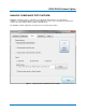
QPHY-SAS3 Software Option TABLE OF CONTENTS INTRODUCTION TO QUALIPHY SAS3 .................................................................................... 5 Required Equipment .................................................................................................................................................. 5 USING QUALIPHY SAS3 .......................................................................................................... 6 QUALIPHY COMPLIANCE TEST PLATFORM ...................
TABLE OF FIGURES Figure 1 - Report menu in QualiPHY General Setup................................................................................ 7 Figure 2 - The Test Report includes a summary table with links to the detailed test results ............. 8 Figure 3 - QualiPHY main menu and compliance test Standard selection menu ............................... 10 Figure 4 - QualiPHY configuration selection menu ...............................................................................
QPHY-SAS3 Software Option INTRODUCTION TO QUALIPHY SAS3 QPHY-SAS3 is an automated software package designed to capture, analyze, and report measurements in conformance with T10 SAS-3 specification as described in the UNH IOL Serial Attached SCSI (SAS) Consortium SAS-3 12Gbps Physical Layer Test Suite (Version 1.0). A copy of the specification can be found on the UNH-IOL FTP site. Note: As of May 19th, 2014 this document can be found at the following site but this is subject to change: ftp://ftp.iol.unh.
USING QUALIPHY SAS3 QualiPHY SAS3 guides the user, step-by-step, through each of the tests in conformance with the T10 SAS-3 specification as described by the UNH-IOL SAS-3 Physical Layer Test suite. To do this, the user must set up a test session. Before beginning testing, users choose the test configuration they wish to run. There are nine pre-loaded test configurations. They are: • 12.0 Gbps Tx tests using Live (Acquisition) Data • 12.
QPHY-SAS3 Software Option QUALIPHY COMPLIANCE TEST PLATFORM QualiPHY is Teledyne LeCroy’s compliance test framework which leads the user through the compliance tests. QualiPHY displays connection diagrams to ensure tests run properly, automates the oscilloscope setup, and generates complete, detailed reports. The QualiPHY software application automates the test and report generation.
See the QualiPHY Operator’s Manual for more information on how to use the QualiPHY framework.
QPHY-SAS3 Software Option Oscilloscope Option Key Installation The required option keys must be purchased to enable the QPHY-SAS3 compliance tests. If you do not have the required option keys already call Teledyne LeCroy Customer Support to place an order and receive the codes. Enter the key and enable the purchased option as follows: 1. From the oscilloscope menu select Utilities Utilities Setup... 2. Select the Options tab and click the Add Key button. 3. Enter the Key Code using the on-screen keyboard.
QualiPHY tests the oscilloscope connection after clicking the Start button. The system prompts you if there is a connection problem. QualiPHY’s Scope Selector function can also be used to verify the connection. Please refer to the QualiPHY Operator’s Manual for explanations on how to use Scope Selector and other QualiPHY functions. Accessing the QPHY-SAS3 Software using QualiPHY This topic provides a basic overview of QualiPHY’s capabilities.
QPHY-SAS3 Software Option 4. Click the Configuration button in the QualiPHY main menu: 5. Select a configuration from the pop-up menu: Figure 4 - QualiPHY configuration selection menu 6. Click Start. 7. Follow the pop-up window prompts.
Customizing QualiPHY The predefined configurations in the Configuration screen cannot be modified. However, you can create your own test configurations by copying one of the standard test configurations and making modifications. A description of the test is also shown in the description field when selected.
QPHY-SAS3 Software Option Creating Custom Configurations Beginning with any of the pre-loaded configurations, 1. Click on the Test Selector tab to change what tests you would like to be included in your new configuration. 2. Click on the Variable Setup tab to change the variables for your new configuration. 3. Click on the Limits tab to change which limit set should be used for your new configuration •See QualiPHY Manual for more information 4.
Figure 6 - Variable Setup and Limits Manager windows 14 922545 Rev A
QPHY-SAS3 Software Option QPHY-SAS3 Operation After pressing Start in the QualiPHY menu, the software instructs how to set up the test using pop-up connection diagrams and dialog boxes. QualiPHY also instructs how to properly configure the DUT to change test signal modes (when necessary).
QPHY-SAS3 TEST CONFIGURATIONS Configurations include variable settings and limit sets as well, not just test selections. See the QPHYSAS3 Variables section for a description of each variable value and its default value. 12.0 Gbps Tx tests using Live (Acquisition) Data This configuration will run all of the tests except for the WDP test and the legacy VMA and VPP tests. The limit set in use is SAS3-12G. All of the variables are set to their default settings except Bitrate is set to 12e9. 12.
QPHY-SAS3 Software Option QPHY-SAS3 VARIABLES Use the Upper (A) or Lower (B) Input For oscilloscope with 2 inputs per channel, this variable allows the user to decide whether to use the A or B input to run the selected tests. The default value for this variable is InputA. Bitrate for SAS3 This variable allows the user to specify the bitrate that is being used for testing. The default value for this variable is 12e9.
Drive Letter for Matlab This variable is used for allows the user to specify the location of the waveforms to be used when running the EyeOpening script remotely over a network. The default value for this variable is D:\. Path to saved Waveforms for offline test This variable allows the user to specify the location of the waveforms to be used when running QPHYSAS3 in Use Saved Data mode. The default value for this variable is D:\Waveforms\SAS3\.
QPHY-SAS3 Software Option QPHY-SAS3 TEST DESCRIPTIONS Tx Group 1 Out of Band Tests 5.1.x (OOB) There are 4 tests run in this group. The tests that are run are: 1. 5.1.1 – Tx Maximum Noise During OOB Idle 2. 5.1.2 – Tx OOB Burst Amplitude 3. 5.1.3 – Tx OOB Offset Delta 4. 5.1.
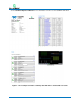
• F8 is a view of the Differential Signal after it has been filtered by the 4.5GHz low-pass Butterworth filter. This is calculated by subtracting the negative input from the positive input. This signal is used to create many of the traces described earlier. Figure 10 - OOB Test Results In the Measure section: • IdleNoise (P1) is the peak-to-peak measurement of F3 (idle differential signal). This is the measured value for Tx – Max Noise During Idle (5.1.1).
QPHY-SAS3 Software Option Tx Group 2 Spread Spectrum Clocking Tests There are 3 tests run in this group. The tests that are run are: 1. 5.2.1 - Tx SSC Modulation Frequency 2. 5.2.2 - Tx SSC Modulation Deviation and Balance 3. 5.2.3 - Tx SSC DFDT (Informative) Each of these 3 tests is run when the DUT is using Center-spreading and Down-Spreading SSC. The purpose of these tests is to verify the SSC Modulation Frequency, Modulation Deviation and Balance and DFDT are within the specification limits.
Figure 12 - SSC Test Results In the Measure section: • Max Freq and Min Freq (P1 and P2) are calculated by measuring the minimum and maximum of the Unfiltered SSCTrack (F3). These are the measured values for Tx - SSC Mod Freq Min and Tx - SSC Mod Freq Max (5.2.2). For 12Gbps these values must be in between +/- 1100 ppm in order to pass this test for center-spreading and -1100 and 100 ppm for down-spreading. For 1.
QPHY-SAS3 Software Option Tx Group 3 (Link Stability, Common Mode, … WDP) There are 7 tests run in this group. The tests that are run are: 1. Tx 5.3.1 Phy Link rate Stability (HFTP) 2. Tx 5.3.2 Common Mode RMS Voltage (CJTPAT) 3. Tx 5.3.4 and 5.3.5 Vpp, VMA, EQ (D30.3) 4. Tx 5.3.6 Rise and Fall Times (HFTP) 5. Tx 5.3.7 RJ, (MFTP, MFTP-SSC-DOWN, MFTP-SSC-CENTER) 6. Tx 5.3.8 TJ, (MFTP, MFTP-SSC-DOWN, MFTP-SSC-CENTER) 7. Tx 5.3.9 Waveform Distortion Penalty Each of these tests are described in detail below.
Figure 14 - Phy Link Rate Stability Test Results In the Measure section: • P1 and P2 are used to calculate the min and the max of F2. These are the measured values for Tx – Min Phy Link Rate Stability (5.3.1) and Tx – Max Phy Link Rate Stability (5.3.1). These values must be between +/- 100ppm in order to pass this test. Tx 5.3.2 Common Mode RMS Voltage (CJTPAT) The purpose of this test is to verify that the common-mode RMS voltage is within the specification limits.
QPHY-SAS3 Software Option Figure 16 - Common Mode RMS Voltage Results In the Measure section: • CM Offset (P1) is the common mode offset. This is measured by taking the mean of the common mode trace. This is the measured value of Tx – Common Mode Offset (5.3.2). This test is informational only. • CM RMS (P2) is the common mode RMS voltage. This is measured by taking the RMS of the common mode trace. This is the measured value for Tx – CM RMS voltage (5.3.2).
• M3 is the Common Mode Spectrum Mask as defined in the specification shown on a linear scale. If the Common Mode Spectrum trace exceeds the mask the test will fail. • F7 is the margin and is calculated as the difference between the Common Mode Spectrum trace and the Common Mode Spectrum Mask. A cursor is placed at 0 dBmV in order to provide a visual aid in seeing where there is positive margin. Figure 18 - Common Mode RMS Voltage Results In the Measure section: • CM Offset (P1) is the common mode offset.
QPHY-SAS3 Software Option Figure 19 - Oscilloscope Configuration after the Vpp, VMA, and EQ tests Shown on this screen: • F2 is Eye Diagram created from the input signal using a 2 pole PLL with a natural frequency of 3.9MHz and a damping factor of .800. This is shown for information only. • F4 is a histogram of the input waveform. • F5 is this histogram converted to a waveform (this is required to perform certain measurements on the histogram). • F6 is the differential input waveform.
• HighMode (P5) is the maximum peak from the right side of the F5. This represents the deemphasized high voltage level of the signal. These are used to calculate the VMA. • VMA (P6) is the difference between the 2 modes of the histogram. This is the measured value of Tx - VMA (5.3.5a). This value must be less than 600mV in order to pass this test. • EQ (P8) is calculated as 20*log10(Vp-p/VMA). This is the measured value of Tx - EQ (5.3.5b). This value must be between 2 and 4 dB in order to pass this test.
QPHY-SAS3 Software Option Figure 22 - Rise and Fall Times Results In the Measure section: • Rise 20-80 (P1) is the 20-80 rise time of the differential input waveform (F1) displayed in ps. This is the measured value of TX - Trise (20-80) (5.3.6). The mean of this value for all rising edges in the differential input must be greater than 20.8 ps in order to pass this test for 12Gbps and greater than 41.6 ps for 1.5Gbps, 3Gbps, and 6Gbps.
Figure 23 - Oscilloscope Configuration after the Rj and Tj Tests Shown on this screen: • F1 is the differential input waveform. • RjBUjHist is the histogram of the random and bounded uncorrelated jitter. This is the same as the full TIE histogram with the DDj removed. The RjBUjHist is an output from SDA III. To comply with the JTF requirements when SSC is not enabled a single-pole PLL is used in SDA III and when SSC is enabled a two-pole PLL is used.
QPHY-SAS3 Software Option Figure 24 - Rj and Tj Results In the SDA Jitter Section: • Tj(1e-12), Rj(spD), Dj(spD), Pj, DCD, and Bitrate are shown. These are all calculations from SDA III. Only the Rj(spD) and Dj(spD) parameters are used for further calculation. The rest of the parameters are informational only. • Rj(spD) is the measured value for Tx - RJ (1-sigma) (5.3.7) using the “spectral direct” method. This is reported as informational only.
At this point that user should run the SASWDP script and enter the returned value in this dialog. By entering this value, the result for the WDP test can be included in the test report provided by QualiPHY. For more information refer to the How to run the SASWDP script section of this manual. After the completion of this test the oscilloscope is in the following configuration: Figure 26 - Oscilloscope Configuration after the WDP Test Shown on this screen: • F1 is the differential input waveform.
QPHY-SAS3 Software Option Tx Group 4 Tx Emphasis There are 3 tests run in this group. The tests that are run are: 1. Tx Emphasis Off (IDLE_REF0) 2. Tx Emphasis Ref1 (IDLE_REF1) 3. Tx Emphasis Ref2 (IDLE_REF2) Each of these tests are described in detail in the following sections. These tests are run when the DUT is outputting IDLE dwords under defined conditions for the precursor, central, and postcursor equalization coefficients with the transmitter set to its maximum peak voltage.
The following figure from the SAS-3 specification provides a definition for the Rpre, Rpost, VMA, and VHL. In each test each of these voltage levels are labeled on the oscilloscope display. Figure 28 – Definition of Rpre, Rpost, VMA, and VHL • • • • 34 Rpre is defined as V3/V2. Rpost is defined as V1/V2. VMA is defined as V2-V5. VHL is defined as the peak to peak voltage on the alternating bit portion of the waveforms.
QPHY-SAS3 Software Option Tx Emphasis Off (IDLE_REF0) The purpose of this test is to gain a reference point in order to compute the equalization calculation for REF1 and REF2. There are no actual pass/fail measurements performed in this test. This test step must be run in order to measure Ref1 or Ref2. This may also be referred to as REF3 or no equalization.
Shown on this screen: • F4 is a plot of the peak voltage values which correspond to V1-V6, VH, and VL. These are the values which are used in the calculation of the first set of Rpre, Rpost, VMA, and VHL values in the Measurement table on the screen. • F6 is a representation of where V1-V6, VH, and VL occur on the acquired waveform. This waveform is an average of all instances where the pattern was identified in the acquired waveform.
QPHY-SAS3 Software Option After the completion of this test the oscilloscope is in the following configuration: Figure 32 - Oscilloscope Configuration after REF1 Test Shown on this screen: • F4 is a plot of the peak voltage values which correspond to V1-V6, VH, and VL. These are the values which are used in the calculation of the first set of Rpre, Rpost, VMA, and VHL values in the Measurement table on the screen. • F6 is a representation of where V1-V6, VH, and VL occur on the acquired waveform.
In the measure section: • Rpre(ML) (P9) is the precursor equalization ratio (Rpre) value which was returned from the SAS3_EYEOPENING script. This is the measured value for TX – Rpre Ref1 (5.4.2.1). This value must be greater than 2.1 and less than 2.97, inclusive. • Rpost(ML) (P10) is the postcursor equalization ratio (Rpost) value which was returned from the SAS3_EYEOPENING script. This is the measured value for TX – Rpost Ref1 (5.4.2.2). This value must be greater than 3 and less than 4, inclusive.
QPHY-SAS3 Software Option After the completion of this test the oscilloscope is in the following configuration: Figure 35 - Oscilloscope Configuration after REF2 Test Shown on this screen: • F4 is a plot of the peak voltage values which correspond to V1-V6, VH, and VL. These are the values which are used in the calculation of the first set of Rpre, Rpost, VMA, and VHL values in the Measurement table on the screen. • F6 is a representation of where V1-V6, VH, and VL occur on the acquired waveform.
In the measure section: • Rpre(ML) (P9) is the precursor equalization ratio (Rpre) value which was returned from the SAS3_EYEOPENING script. This is the measured value for TX – Rpre Ref1 (5.4.2.1). This value must be greater than 1.05 and less than 1.49, inclusive. • Rpost(ML) (P10) is the postcursor equalization ratio (Rpost) value which was returned from the SAS3_EYEOPENING script. This is the measured value for TX – Rpost Ref1 (5.4.2.2). This value must be greater than 1.19 and less than 1.68, inclusive.
QPHY-SAS3 Software Option HOW TO RUN THE SASWDP SCRIPT The SASWDP script is required for running the Waveform Distortion Penalty (5.3.9) test. This script can be obtained from the T10 organization website (http://www.t10.org/cgi-bin/ac.pl). A valid T10 login is required for downloading this download. Note: As of March 2nd, 2014 this script can be found at the following site but this is subject to change: http://www.t10.org/cgi-bin/ac.pl?t=d&f=09-015r0.zip 1.
5. Enter the value for xWDP that is returned from the SASWDP screen in the dialog box described in the Tx 5.3.9 Waveform Distortion Penalty description above.
QPHY-SAS3 Software Option HOW TO RUN THE SAS3_EYEOPENING SCRIPT The SAS3_EYEOPENING script is required to process the results for the Group 4 Tx Emphasis tests. This script is included with the QPHY-SAS3 software but can also be obtained from the T10 organization website. The SAS3_EYEOPENING script requires a registered version of Matlab. A Matlab license can either be installed on the oscilloscope or can be run from a separate PC.
APPENDIX A: CABLE DESKEWING There is an automatic cable deskew wizard built in to QPHY-SAS3. When the variable Test Mode is set to Yes then deskew wizard will prompt the user before the making the first acquisition. Note: Cables should be deskewed once the temperature of the oscilloscope is stable. The oscilloscope must be warmed up for about twenty at least a half-hour before proceeding. This procedure should be run again if the temperature of the oscilloscope changes by more than a few degrees.
QPHY-SAS3 Software Option Using Fast Edge The Fast Edge deskew technique will use the Fast Edge output on the oscilloscope to deskew C2 and C3. The first step is to connect C2 to the Fast Edge connection on the oscilloscope. The connection to C2 should the cables and DC blocks which will be used during the testing. Figure 40 – Fast Edge – Step 1 Prompt Before moving on to Step 2 the display on the oscilloscope screen should appear as below. F2 is setup to be used for the deskew calculation of C2.
The second step is to disconnect C2 from the Fast Edge and connect C3. The connection to C3 should the cables and DC blocks which will be used during the testing. Figure 42 – Fast Edge – Step 2 Prompt Before moving on to Step 3 the display on the oscilloscope screen should appear as below. F2 has been saved to M2 and F3 is setup to be used for the deskew calculation of C3.
QPHY-SAS3 Software Option At this point the C2 and C3 can both be reconnected to the test fixture. Figure 44 – Fast Edge – Step 3 Prompt Before completing the deskew process the display on the oscilloscope screen should appear as below. F2 has been saved to M2 and has been saved to M3. The skew between M2 and M3 is calculated in P1. This is the skew value which will be used during the testing. This value is stored in QPHY-SAS3 and it is not necessary to re-run this process every time you run QPHY-SAS3.
Using MFTP from DUT The MFTP deskew technique will use the DUT to provide an MFTP signal to C2 and C3 in order to deskew both channels. The first step is to connect C2 to Txp on the DUT and C3 to Txn on the DUT. The DUT should be configured to output a MFTP pattern. The connections to C2 and C3 should include the cables and DC blocks which will be used during the testing. Figure 46 – MFTP – Step 1 Prompt Before moving on to Step 2 the display on the oscilloscope screen should appear as below.
QPHY-SAS3 Software Option The second step is to swap Txp and Txn at the device side. Figure 48 – MFTP – Step 2 Prompt Before moving on to Step 3 the display on the oscilloscope screen should appear as below. C3 has been inverted and both C2 and C3 has been rescaled. The skew between C2 and C3 is calculated in P1. This is the skew value which will be used during the testing. This value is stored in QPHY-SAS3 and it is not necessary to re-run this process every time you run QPHY-SAS3.
APPENDIX B: FILE NAME CONVENTIONS FOR SAVED WAVEFORM DATA When live tests are made, the acquired waveforms are stored using these file names. If there is data which has been already acquired, to perform tests using this package, the files must be renamed to conform to these conventions: Please note (at this time) there is no distinction between bit rates, so please use different folders for results at 12, 6, 3, and 1.5 Gbps.