TI-84 Plus and TI-84 Plus Silver Edition Guidebook Note: This guidebook for the TI-84 Plus or TI-84 Plus Silver Edition with operating system (OS) version 2.55MP. If your calculator has a previous OS version, your screens may look different and some features may not be available. You can download the latest OS education.ti.com/guides.
Important Information Texas Instruments makes no warranty, either express or implied, including but not limited to any implied warranties of merchantability and fitness for a particular purpose, regarding any programs or book materials and makes such materials available solely on an "as-is" basis.
Contents Important Information .................................................................................................................... ii Chapter 1: Operating the TI-84 Plus Silver Edition .................................................................... 1 Documentation Conventions .......................................................................................................... 1 TI-84 Plus Keyboard ...................................................................................
Chapter 4: Parametric Graphing .............................................................................................. 91 Getting Started: Path of a Ball ...................................................................................................... 91 Defining and Displaying Parametric Graphs ................................................................................ 93 Exploring Parametric Graphs ...........................................................................................
Horiz (Horizontal) Split Screen .................................................................................................... 139 G-T (Graph-Table) Split Screen .................................................................................................... 140 TI-84 Plus Pixels in Horiz and G-T Modes .................................................................................... 141 Chapter 10: Matrices .......................................................................................
Getting Started: Financing a Car ................................................................................................ 252 Getting Started: Computing Compound Interest ...................................................................... 253 Using the TVM Solver ................................................................................................................. 253 Using the Financial Functions .........................................................................................
Resetting the TI-84 Plus ............................................................................................................... 333 Grouping and Ungrouping Variables ......................................................................................... 336 Garbage Collection ...................................................................................................................... 339 ERR:ARCHIVE FULL Message ............................................................................
Chapter 1: Operating the TI-84 Plus Silver Edition Documentation Conventions In the body of this guidebook, TI-84 Plus refers to the TI-84 Plus Silver Edition, but all of the instructions, examples, and functions in this guidebook also work for the TI-84 Plus. The two graphing calculators differ only in available RAM memory, interchangeable faceplates, and Flash application ROM memory. Sometimes, as in Chapter 19, the full name TI-84 Plus Silver Edition is used to distinguish it from the TI-84 Plus.
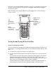
TI-84 Plus Silver Edition Graphing Keys Editing Keys Advanced Function Keys Scientific Calculator Keys Using the Color.Coded Keyboard The keys on the TI-84 Plus are color-coded to help you easily locate the key you need. The light colored keys are the number keys. The keys along the right side of the keyboard are the common math functions. The keys across the top set up and display graphs.
If you want to enter several alphabetic characters in a row, you can press y 7 to lock the alpha key in the On position and avoid having to press ƒ multiple times. Press ƒ a second time to unlock it. Note: The flashing cursor changes to Ø when you press ƒ, even if you are accessing a function or a menu. ƒ^-a y Accesses the second function printed above each key. Access shortcut menus for functionality including templates for fractions, n/d, and other functions.
• If the TI-84 Plus is turned off and connected to another graphing calculator or personal computer, any communication activity will “wake up” the TI-84 Plus. To prolong the life of the batteries, APD™ turns off the TI-84 Plus automatically after about five minutes without any activity. Turning Off the Graphing Calculator To turn off the TI-84 Plus manually, press y M. • All settings and memory contents are retained by the Constant Memory™ function. • Any error condition is cleared.
Generally, the graphing calculator will continue to operate for one or two weeks after the lowbattery message is first displayed. After this period, the TI-84 Plus will turn off automatically and the unit will not operate. Batteries must be replaced. All memory should be retained. Note: • The operating period following the first low-battery message could be longer than two weeks if you use the graphing calculator infrequently.
When an entry is executed on the home screen, the answer is displayed on the right side of the next line. Entry Answer The mode settings control the way the TI-84 Plus interprets expressions and displays answers. If an answer, such as a list or matrix, is too long to display entirely on one line, an arrow (MathPrint™) or an ellipsis (Classic) is displayed to the right or left. Press ~ and | to display the answer.
• Templates to enter fractions and selected functions from the MATH MATH and MATH NUM menus as you would see them in a textbook. Functions include absolute value, summation, numeric differentiation, numeric integration, and log base n. • Matrix entry. • Names of function variables from the VARS Y-VARS menu. Initially, the menus are hidden. To open a menu, press t plus the F-key that corresponds to the menu, that is, ^ for FRAC, _ for FUNC, ` for MTRX, or a for YVAR.
Busy Indicator When the TI-84 Plus is calculating or graphing, a vertical moving line is displayed as a busy indicator in the top-right corner of the screen. When you pause a graph or a program, the busy indicator becomes a vertical moving dotted line. Display Cursors In most cases, the appearance of the cursor indicates what will happen when you press the next key or select the next menu item to be pasted as a character.
Removing a Faceplate 1. Lift the tab at the bottom edge of the faceplate away from the TI-84 Plus Silver Edition case. 2. Carefully lift the faceplate away from the unit until it releases. Be careful not to damage the faceplate or the keyboard. Installing New Faceplates 1. Align the top of the faceplate in the corresponding grooves of the TI-84 Plus Silver Edition case. 2. Gently click the faceplate into place. Do not force. 3.
Changing the Clock Settings 1. Press the ~ or | to highlight the date format you want. Press Í. 2. Press † to highlight YEAR. Press ‘ and type the year. 3. Press † to highlight MONTH. Press ‘ and type the number of the month (1-12). 4. Press † to highlight DAY. Press ‘ and type the date. 5. Press † to highlight TIME. Press ~ or | to highlight the time format you want. Press Í. 6. Press † to highlight HOUR. Press ‘ and type the hour (a number from 1-12 or 0-23). 7. Press † to highlight MINUTE.
Using the Mode Screen to turn the clock on 1. If the clock is turned off, Press † to highlight TURN CLOCK ON. 2. Press Í Í. Using the Catalog to turn the clock on 1. If the clock is turned off, Press y N 2. Press † or } to scroll the CATALOG until the selection cursor points to ClockOn. 3. Press Í Í. Turning the Clock Off 1. Press y N. 2. Press † or } to scroll the CATALOG until the selection cursor points to ClockOff. 3. Press Í Í.
Entering an Expression To create an expression, you enter numbers, variables, and functions using the keyboard and menus. An expression is completed when you press Í, regardless of the cursor location. The entire expression is evaluated according to Equation Operating System (EOS™) rules, and the answer is displayed according to the mode setting for Answer. Most TI-84 Plus functions and operations are symbols comprising several characters.
Note: The Catalog Help App contains syntax information for most of the functions in the catalog. Instructions An instruction initiates an action. For example, ClrDraw is an instruction that clears any drawn elements from a graph. Instructions cannot be used in expressions. In general, the first letter of each instruction name is uppercase. Some instructions take more than one argument, as indicated by an open parenthesis at the end of the name.
Keystrokes Result { Deletes a character at the cursor; this key repeats. y6 Changes the cursor to an underline (__); inserts characters in front of the underline cursor; to end insertion, press y 6 or press |, }, ~, or †. y Changes the cursor to Þ; the next keystroke performs a 2nd function (displayed above a key and to the left); to cancel 2nd, press y again.
GoTo Format Graph: No Yes Shortcut to the Format Graph screen (y .) StatDiagnostics: Off On Determines which information is displayed in a statistical regression calculation StatWizards: On Off Determines if syntax help prompts are provided for optional and required arguments for many statistical, regression and distribution commands and functions.
Sci (scientific) notation mode expresses numbers in two parts. The significant digits display with one digit to the left of the decimal. The appropriate power of 10 displays to the right of å, as in 1.234567â4. Eng (engineering) notation mode is similar to scientific notation. However, the number can have one, two, or three digits before the decimal; and the power-of-10 exponent is a multiple of three, as in 12.34567â3.
Seq (sequence) graphing mode plots sequences (Chapter 6). Connected, Dot Connected plotting mode draws a line connecting each point calculated for the selected functions. Dot plotting mode plots only the calculated points of the selected functions. Sequential, Simul Sequential graphing-order mode evaluates and plots one function completely before the next function is evaluated and plotted.
• Horiz (horizontal) mode displays the current graph on the top half of the screen; it displays the home screen or an editor on the bottom half (Chapter 9). • G-T (graph-table) mode displays the current graph on the left half of the screen; it displays the table screen on the right half (Chapter 9). MathPrint™, Classic MathPrint™ mode displays most inputs and outputs the way they are shown in textbooks, such as 2 1 3 --- + --- and ∫ x 2 dx .
Yes leaves the mode screen and displays the FORMAT graph screen when you press Í so that you can change the graph format settings. To return to the mode screen, press z. Stat Diagnostics: Off, On Off displays a statistical regression calculation without the correlation coefficient (r) or the coefficient of determination (r2). On displays a statistical regression calculation with the correlation coefficient (r), and the coefficient of determination (r2), as appropriate.
Variable Type Names Polar functions r1, r2, r3, r4, r5, r6 Sequence functions u, v, w Stat plots Plot1, Plot2, Plot3 Graph databases GDB1, GDB2, ... , GDB9, GDB0 Graph pictures Pic1, Pic2, ... , Pic9, Pic0 Strings Str1, Str2, ... , Str9, Str0 Apps Applications AppVars Application variables Groups Grouped variables System variables Xmin, Xmax, and others Notes about Variables • You can create as many list names as memory will allow (Chapter 11).
3. Press ƒ and then the letter of the variable to which you want to store the value. 4. Press Í. If you entered an expression, it is evaluated. The value is stored to the variable. Displaying a Variable Value To display the value of a variable, enter the name on a blank line on the home screen, and then press Í. Archiving Variables (Archive, Unarchive) You can archive data, programs, or other variables in a section of memory called user data archive where they cannot be edited or deleted inadvertently.
3. Press Í. The variable contents are inserted where the cursor was located before you began these steps. Note: You can edit the characters pasted to the expression without affecting the value in memory. Scrolling Through Previous Entries on the Home Screen You can scroll up through previous entries and answers on the home screen, even if you have cleared the screen. When you find an entry or answer that you want to use, you can select it and paste it on the current entry line.
Because the TI-84 Plus updates ENTRY only when you press Í, you can recall the previous entry even if you have begun to enter the next expression. 5Ã7 Í y[ Accessing a Previous Entry The TI-84 Plus retains as many previous entries as possible in ENTRY, up to a capacity of 128 bytes. To scroll those entries, press y [ repeatedly. If a single entry is more than 128 bytes, it is retained for ENTRY, but it cannot be placed in the ENTRY storage area.
When you press y [, all the expressions and instructions separated by colons are pasted to the current cursor location. You can edit any of the entries, and then execute all of them when you press Í. Example: For the equation A=pr 2, use trial and error to find the radius of a circle that covers 200 square centimeters. Use 8 as your first guess. 8 ¿ ƒ R ƒ ã :ä yB ƒ R ¡Í y[ y | 7 y 6 Ë 95 Í Continue until the answer is as accurate as you want.
Continuing an Expression You can use Ans as the first entry in the next expression without entering the value again or pressing y Z. On a blank line on the home screen, enter the function. The TI-84 Plus pastes the variable name Ans to the screen, then the function. 5¥2 Í ¯9Ë9 Í Storing Answers To store an answer, store Ans to a variable before you evaluate another expression. Calculate the area of a circle of radius 5 meters. Next, calculate the volume of a cylinder of radius 5 meters and height 3.
Displaying a Menu While using your TI-84 Plus, you often will need to access items from its menus. When you press a key that displays a menu, that menu temporarily replaces the screen where you are working. For example, when you press , the MATH menu is displayed as a full screen. After you select an item from a menu, the screen where you are working usually is displayed again. Moving from One Menu to Another Some keys access more than one menu.
Selecting an Item from a Menu You can select an item from a menu in either of two ways. • Press the number or letter of the item you want to select. The cursor can be anywhere on the menu, and the item you select need not be displayed on the screen. • Press † or } to move the cursor to the item you want, and then press Í. After you select an item from a menu, the TI-84 Plus typically displays the previous screen.
To display the VARS menu, press . All VARS menu items display secondary menus, which show the names of the system variables. 1:Window, 2:Zoom, and 5:Statistics each access more than one secondary menu. VARS Y-VARS 1: Window... X/Y, T/q, and U/V/W variables 2: Zoom... ZX/ZY, ZT/Zq, and ZU variables 3: GDB... Graph database variables 4: Picture... Picture variables 5: Statistics... XY, G, EQ, TEST, and PTS variables 6: Table... TABLE variables 7: String...
Equation Operating System (EOS™) Order of Evaluation The Equation Operating System (EOS™) defines the order in which functions in expressions are entered and evaluated on the TI-84 Plus. EOS™ lets you enter numbers and functions in a simple, straightforward sequence. EOS™ evaluates the functions in an expression in this order.
Negation To enter a negative number, use the negation key. Press Ì and then enter the number. On the TI-84 Plus, negation is in the third level in the EOS™ hierarchy. Functions in the first level, such as squaring, are evaluated before negation. Example: MX2, evaluates to a negative number (or 0). Use parentheses to square a negative number. Note: Use the ¹ key for subtraction and the Ì key for negation.
Archiving You can store variables in the TI-84 Plus user data archive, a protected area of memory separate from RAM. The user data archive lets you: • Store data, programs, applications or any other variables to a safe location where they cannot be edited or deleted inadvertently. • Create additional free RAM by archiving variables. By archiving variables that do not need to be edited frequently, you can free up RAM for applications that may require additional memory. For details, refer to: Chapter 18.
Lists You can enter and save as many lists as memory allows for use in statistical analyses. You can attach formulas to lists for automatic computation. You can use lists to evaluate expressions at multiple values simultaneously and to graph a family of curves. For details, refer to:Chapter 11. Statistics You can perform one- and two-variable, list-based statistical analyses, including logistic and sine regression analysis.
Archiving Archiving allows you to store data, programs, or other variables to user data archive where they cannot be edited or deleted inadvertently. Archiving also allows you to free up RAM for variables that may require additional memory. Archived variables are indicated by asterisks (ä) to the left of the variable names. For details, refer to Chapter 16.
• If you select 1:Quit (or press y 5 or ‘), then the home screen is displayed. • If you select 2:Goto, then the previous screen is displayed with the cursor at or near the error location. Note: If a syntax error occurs in the contents of a Y= function during program execution, then the Goto option returns to the Y= editor, not to the program. Correcting an Error To correct an error, follow these steps. 1. Note the error type (ERR:error type). 2. Select 2:Goto, if it is available.
Chapter 2: Math, Angle, and Test Operations Getting Started: Coin Flip Getting Started is a fast-paced introduction. Read the chapter for details. For more probability simulations, try the Probability Simulations App for the TI-84 Plus. You can download this App from education.ti.com. Suppose you want to model flipping a fair coin 10 times. You want to track how many of those 10 coin flips result in heads. You want to perform this simulation 40 times.
Keyboard Math Operations Using Lists with Math Operations Math operations that are valid for lists return a list calculated element by element. If you use two lists in the same expression, they must be the same length. Addition, Subtraction, Multiplication, Division You can use + (addition, Ã), N (subtraction, ¹), … (multiplication, ¯), and à (division, ¥) with real and complex numbers, expressions, lists, and matrices. You cannot use à with matrices. If you need to input A/2, enter this as A †1/2 or A †.
Inverse You can use L1 (inverse, œ) with real and complex numbers, expressions, lists, and matrices. The multiplicative inverse is equivalent to the reciprocal, 1àx. value-1 log(, 10^(, ln( You can use log( (logarithm, «), 10^( (power of 10, y G), and ln( (natural log, μ) with real or complex numbers, expressions, and lists. log(value) MathPrint™: 10power Classic: 10^(power) ln(value) Exponential e^( (exponential, y J) returns the constant e raised to a power.
Mvalue EOS™ rules (Chapter 1) determine when negation is evaluated. For example, L42 returns a negative number, because squaring is evaluated before negation. Use parentheses to square a negated number, as in (L4)2. Note: On the TI-84 Plus, the negation symbol (M) is shorter and higher than the subtraction sign (N), which is displayed when you press ¹. Pi p (Pi, y B) is stored as a constant in the TI-84 Plus. In calculations, the TI-84 Plus uses 3.1415926535898 for p.
MATH NUM CPX PRB Computes the function integral. 9: fnInt( 0: summation A: logBASE( Returns the logarithm of a specifed value determined from a specified base: logBASE(value, base). B: Solver... Displays the equation solver. )( Returns the sum of elements of list from start to end, where start <= end. 4Frac, 4Dec 4Frac (display as a fraction) displays an answer as its rational equivalent. You can use 4Frac with real or complex numbers, expressions, lists, and matrices.
x‡ (Root) x ‡ (xth root) returns the xth root of value. You can use x‡ with real or complex numbers, expressions, and lists. xthrootx‡value fMin(, fMax( fMin( (function minimum) and fMax( (function maximum) return the value at which the local minimum or local maximum value of expression with respect to variable occurs, between lower and upper values for variable. fMin( and fMax( are not valid in expression. The accuracy is controlled by tolerance (if not specified, the default is 1âL5).
MathPrint™: Classic: nDeriv(expression,variable,value[,H]) nDeriv( uses the symmetric difference quotient method, which approximates the numerical derivative value as the slope of the secant line through these points. ( x + ε ) – f ( x – ε )f′ ( x ) = f----------------------------------------2ε As H becomes smaller, the approximation usually becomes more accurate. In MathPrint™ mode, the default H is 1EM3. You can switch to Classic mode to change H for investigations.
Note: To speed the drawing of integration graphs (when fnInt( is used in a Y= equation), increase the value of the Xres window variable before you press s. Using the Equation Solver Solver Solver displays the equation solver, in which you can solve for any variable in an equation. The equation is assumed to be equal to zero. Solver is valid only for real numbers. When you select Solver, one of two screens is displayed.
• The default lower and upper bounds appear in the last line of the editor (bound={L1â99,1â99}). • A $ is displayed in the first column of the bottom line if the editor continues beyond the screen. Note: To use the solver to solve an equation such as K=.5MV2, enter eqn:0=KN.5MV2 in the equation editor. Entering and Editing Variable Values When you enter or edit a value for a variable in the interactive solver editor, the new value is stored in memory to that variable.
3. Enter an initial guess for the variable for which you are solving. This is optional, but it may help find the solution more quickly. Also, for equations with multiple roots, the TI-84 Plus will attempt to display the solution that is closest to your guess. ( upper + lower ) The default guess is calculated as ----------------------------------------- . 2 4. Edit bound={lower,upper}. lower and upper are the bounds between which the TI-84 Plus searches for a solution.
squares next to the previous solution and leftNrt=diff disappear. Move the cursor to the variable for which you now want to solve and press ƒ \. Controlling the Solution for Solver or solve( The TI-84 Plus solves equations through an iterative process. To control that process, enter bounds that are relatively close to the solution and enter an initial guess within those bounds. This will help to find a solution more quickly. Also, it will define which solution you want for equations with multiple solutions.
MATH NUM CPX PRB 4: fPart( Fractional part 5: int( Greatest integer 6: min( Minimum value 7: max( Maximum value 8: lcm( Least common multiple 9: gcd( Greatest common divisor 0: remainder( Reports the remainder as a whole number from a division of two A: 4n/d3 4Un/d Converts an improper fraction to a mixed number or a mixed number to an improper fraction. B: 4F3 4D Converts a decimal to a fraction or a fraction to a decimal.
round( round( returns a number, expression, list, or matrix rounded to #decimals (9). If #decimals is omitted, value is rounded to the digits that are displayed, up to 10 digits. round(value[,#decimals]) iPart(, fPart( iPart( (integer part) returns the integer part or parts of real or complex numbers, expressions, lists, and matrices. iPart(value) fPart( (fractional part) returns the fractional part or parts of real or complex numbers, expressions, lists, and matrices.
Note: For a given value, the result of int( is the same as the result of iPart( for nonnegative numbers and negative integers, but one integer less than the result of iPart( for negative noninteger numbers. min(, max( min( (minimum value) returns the smaller of valueA and valueB or the smallest element in list. If listA and listB are compared, min( returns a list of the smaller of each pair of elements. If list and value are compared, min( compares each element in list with value.
remainder( remainder( returns the remainder resulting from the division of two positive whole numbers, dividend and divisor, each of which can be a list. The divisor cannot be zero. If both arguments are lists, they must have the same number of elements. If one argument is a list and the other a non-list, the nonlist is paired with each element of the list, and a list is returned.
4F3 4D 4F3 4D converts a fraction to a decimal or a decimal to a fraction. You can also access 4F3 4D from the FRAC shortcut menu (t ^ 4). Un/d Un/d displays the mixed number template. You can also access Un/d from the FRAC shortcut menu (t ^ 2). In the fraction, n and d must be non-negative integers. MathPrint™ " Classic n/d n/d displays the mixed number template. You can also access n/d from the FRAC shortcut menu (t ^ 1). n and d can be real numbers or expressions but may not contain complex numbers.
On the TI-84 Plus, complex numbers can be stored to variables. Also, complex numbers are valid list elements. In Real mode, complex-number results return an error, unless you entered a complex number as input. For example, in Real mode ln(L1) returns an error; in a+bi mode ln(L1) returns an answer. Real mode a+bi mode $ $ Entering Complex Numbers Complex numbers are stored in rectangular form, but you can enter a complex number in rectangular form or polar form, regardless of the mode setting.
Note about Radian Versus Degree Mode Radian mode is recommended for complex number calculations. Internally, the TI-84 Plus converts all entered trigonometric values to radians, but it does not convert values for exponential, logarithmic, or hyperbolic functions. In degree mode, complex identities such as e^(iq) = cos(q) + i sin(q) are not generally true because the values for cos and sin are converted to radians, while those for e^() are not.
To enter a complex number in polar form, enter the value of r (magnitude), press y J (exponential function), enter the value of q (angle), press y V (constant), and then press ¤.
MATH CPX (Complex) Operations MATH CPX Menu To display the MATH CPX menu, press ~ ~. MATH NUM CPX PRB 1: conj( Returns the complex conjugate. 2: real( Returns the real part. 3: imag( Returns the imaginary part. 4: angle( Returns the polar angle. 5: abs( Returns the magnitude (modulus). 6: 4Rect Displays the result in rectangular form. 7: 4Polar Displays the result in polar form. conj( conj( (conjugate) returns the complex conjugate of a complex number or list of complex numbers.
imag( imag( (imaginary part) returns the imaginary (nonreal) part of a complex number or list of complex numbers. imag(a+bi) returns b. imag(re^(qi)) returns r†sin(q). MathPrint™ Classic angle( angle( returns the polar angle of a complex number or list of complex numbers, calculated as tanL1 (b/a), where b is the imaginary part and a is the real part. The calculation is adjusted by +p in the second quadrant or Np in the third quadrant. angle(a+bi) returns tanL1(b/a).
abs(a+bi) returns . abs(re^(qi)) returns r (magnitude). 4Rect 4Rect (display as rectangular) displays a complex result in rectangular form. It is valid only at the end of an expression. It is not valid if the result is real. complex result8Rect returns a+bi. 4Polar 4Polar (display as polar) displays a complex result in polar form. It is valid only at the end of an expression. It is not valid if the result is real. complex result8Polar returns re^(qi).
MATH NUM CPX PRB 2: nPr Number of permutations 3: nCr Number of combinations 4: ! Factorial 5: randInt( Random-integer generator 6: randNorm( Random # from Normal distribution 7: randBin( Random # from Binomial distribution 8: randIntNoRep( Random ordered list of integers in a range rand rand (random number) generates and returns one or more random numbers > 0 and < 1. To generate a list of random-numbers, specify an integer > 1 for numtrials (number of trials).
Factorial ! (factorial) returns the factorial of either an integer or a multiple of .5. For a list, it returns factorials for each integer or multiple of .5. value must be ‚ L.5 and 69. value! Note: The factorial is computed recursively using the relationship (n+1)! = n…n!, until n is reduced to either 0 or L1/2. At that point, the definition 0!=1 or the definition (L1à2)!=‡p is used to complete the calculation. Hence: n!=n…(nN1)…(nN2)… ... …2…1, if n is an integer ‚ 0 n!= n…(nN1)…(nN2)… ...
randBin( randBin( (random Binomial) generates and displays a random integer from a specified Binomial distribution. numtrials (number of trials) must be ‚ 1. prob (probability of success) must be ‚ 0 and 1. To generate a list of random numbers, specify an integer > 1 for numsimulations (number of simulations); if not specified, the default is 1. randBin(numtrials,prob[,numsimulations]) Note: The seed value stored to rand also affects randInt(, randNorm(, and randBin( instructions.
ANGLE 3: r Radian notation 4: 8DMS Displays as degree/minute/second 5: R8Pr( Returns r, given X and Y 6: R8Pq( 7: P8Rx( Returns x, given R and q 8: P8Ry( Returns y, given R and q Returns q, given X and Y Entry Notation DMS (degrees/minutes/seconds) entry notation comprises the degree symbol (¡), the minute symbol ('), and the second symbol ("). degrees must be a real number; minutes and seconds must be real numbers ‚ 0.
Radians r (radians) designates an angle or list of angles as radians, regardless of the current angle mode setting. In Degree mode, you can use r to convert radians to degrees. valuer Degree mode 8DMS 8DMS (degree/minute/second) displays answer in DMS format. The mode setting must be Degree for answer to be interpreted as degrees, minutes, and seconds. 8DMS is valid only at the end of a line.
TEST (Relational) Operations TEST Menu To display the TEST menu, press y :. This operator... TEST Returns 1 (true) if... LOGIC 1: = Equal 2: ƒ Not equal to 3: > Greater than 4: ‚ Greater than or equal to 5: < Less than 6: Less than or equal to Ä=, ƒ, >, ‚, <, Relational operators compare valueA and valueB and return 1 if the test is true or 0 if the test is false. valueA and valueB can be real numbers, expressions, or lists.
TEST LOGIC (Boolean) Operations TEST LOGIC Menu To display the TEST LOGIC menu, press y : ~. This operator... TEST Returns a 1 (true) if... LOGIC 1: and Both values are nonzero (true). 2: or At least one value is nonzero (true). 3: xor Only one value is zero (false). 4: not( The value is zero (false). Boolean Operators Boolean operators are often used in programs to control program flow and in graphing to control the graph of the function over specific values.
Boolean logic is often used with relational tests. In the following program, the instructions store 4 into C.
Chapter 3: Function Graphing Getting Started: Graphing a Circle Getting Started is a fast-paced introduction. Read the chapter for details. Graph a circle of radius 10, centered on the origin in the standard viewing window. To graph this circle, you must enter separate formulas for the upper and lower portions of the circle. Then use ZSquare (zoom square) to adjust the display and make the functions appear as a circle. 1. In Func mode, press o to display the Y= editor.
4. To see the ZSquare window variables, press p and notice the new values for Xmin, Xmax, Ymin, and Ymax. Defining Graphs TI-84 Plus—Graphing Mode Similarities Chapter 3 specifically describes function graphing, but the steps shown here are similar for each TI-84 Plus graphing mode. Chapters 4, 5, and 6 describe aspects that are unique to parametric graphing, polar graphing, and sequence graphing. Defining a Graph To define a graph in any graphing mode, follow these steps.
You can store a picture of the current graph display to any of 10 graph picture variables (Pic1 through Pic9, and Pic0; Chapter 8). Then you can superimpose one or more stored pictures onto the current graph. Setting the Graph Modes Checking and Changing the Graphing Mode To display the mode screen, press z. The default settings are highlighted below. To graph functions, you must select Func mode before you enter values for the window variables and before you enter the functions.
Defining Functions Displaying Functions in the Y= Editor To display the Y= editor, press o. You can store up to 10 functions to the function variables Y1 through Y9, and Y0. You can graph one or more defined functions at once. In this example, functions Y1 and Y2 are defined and selected. Defining or Editing a Function To define or edit a function, follow these steps. 1. Press o to display the Y= editor. 2. Press † to move the cursor to the function you want to define or edit. To erase a function, press ‘.
3. Press ƒ a to display the YVAR shortcut menu, move the cursor to the function name, and then press Í. "expression"!Yn When the instruction is executed, the TI-84 Plus stores the expression to the designated variable Yn, selects the function, and displays the message Done. Evaluating Y= Functions in Expressions You can calculate the value of a Y= function Yn at a specified value of X. A list of values returns a list. Yn(value) Yn({value1,value2,value3, . . .
Turning On or Turning Off a Stat Plot in the Y= Editor To view and change the on/off status of a stat plot in the Y= editor, use Plot1 Plot2 Plot3 (the top line of the Y= editor). When a plot is on, its name is highlighted on this line. To change the on/off status of a stat plot from the Y= editor, press } and ~ to place the cursor on Plot1, Plot2, or Plot3, and then press Í. Plot1 is turned on. Plot2 and Plot3 are turned off.
Setting Graph Styles for Functions MATH Graph Style Icons in the Y= Editor This table describes the graph styles available for function graphing. Use the styles to visually differentiate functions to be graphed together. For example, you can set Y1 as a solid line, Y2 as a dotted line, and Y3 as a thick line.
Shading Above and Below When you select é or ê for two or more functions, the TI-84 Plus rotates through four shading patterns. • Vertical lines shade the first function with a é or ê graph style. • Horizontal lines shade the second. • Negatively sloping diagonal lines shade the third. • Positively sloping diagonal lines shade the fourth. • The rotation returns to vertical lines for the fifth é or ê function, repeating the order described above. When shaded areas intersect, the patterns overlap.
Setting the Viewing Window Variables The TI-84 Plus Viewing Window The viewing window is the portion of the coordinate plane defined by Xmin, Xmax, Ymin, and Ymax. Xscl (X scale) defines the distance between tick marks on the x-axis. Yscl (Y scale) defines the distance between tick marks on the y-axis. To turn off tick marks, set Xscl=0 and Yscl=0. Displaying the Window Variables To display the current window variable values, press p.
1. Enter the value you want to store. 2. Press ¿. 3. Press to display the VARS menu. 4. Select 1:Window to display the Func window variables (X/Y secondary menu). • Press ~ to display the Par and Pol window variables (T/q secondary menu). • Press ~ ~ to display the Seq window variables (U/V/W secondary menu). 5. Select the window variable to which you want to store a value. The name of the variable is pasted to the current cursor location. 6. Press Í to complete the instruction.
AxesOn LabelOff ExprOn AxesOff LabelOn ExprOff Sets axes on or off. Sets axes label off or on. Sets expression display on or off. Format settings define a graph’s appearance on the display. Format settings apply to all graphing modes. Seq graphing mode has an additional mode setting (Chapter 6). Changing a Format Setting To change a format setting, follow these steps. 1. Press †, ~, }, and | as necessary to move the cursor to the setting you want to select. 2. Press Í to select the highlighted setting.
AxesOff does not display the axes. This overrides the LabelOff/ LabelOn format setting. LabelOff, LabelOn LabelOff and LabelOn determine whether to display labels for the axes (X and Y), if AxesOn format is also selected. ExprOn, ExprOff ExprOn and ExprOff determine whether to display the Y= expression when the trace cursor is active. This format setting also applies to stat plots. When ExprOn is selected, the expression is displayed in the top-left corner of the graph screen.
• Changed the value of a variable in a selected function • Changed a window variable or graph format setting • Cleared drawings by selecting ClrDraw • Changed a stat plot definition Overlaying Functions on a Graph On the TI-84 Plus, you can graph one or more new functions without replotting existing functions. For example, store sin(X) to Y1 in the Y= editor and press s. Then store cos(X) to Y2 and press s again. The function Y2 is graphed on top of Y1, the original function.
Exploring Graphs with the Free-Moving Cursor Free-Moving Cursor When a graph is displayed, press |, ~, }, or † to move the cursor around the graph. When you first display the graph, no cursor is visible. When you press |, ~, }, or †, the cursor moves from the center of the viewing window. As you move the cursor around the graph, the coordinate values of the cursor location are displayed at the bottom of the screen if CoordOn format is selected.
Moving the Trace Cursor To move the TRACE cursor do this: To the previous or next plotted point, press | or ~. Five plotted points on a function (Xres affects this), press y | or y ~. To any valid X value on a function, enter a value, and then press Í. From one function to another, press } or †. When the trace cursor moves along a function, the Y value is calculated from the X value; that is, Y=Yn(X). If the function is undefined at an X value, the Y value is blank.
Panning to the Left or Right If you trace a function beyond the left or right side of the screen, the viewing window automatically pans to the left or right. Xmin and Xmax are updated to correspond to the new viewing window. Quick Zoom While tracing, you can press Í to adjust the viewing window so that the cursor location becomes the center of the new viewing window, even if the cursor is above or below the display. This allows panning up and down. After Quick Zoom, the cursor remains in TRACE.
ZOOM MEMORY B: ZFrac1/2 Sets the window variables so that you can trace in increments of , if possible. Sets @X and @Y to C: ZFrac1/3 . Sets the window variables so that you can trace in increments of , if possible. Sets @X and @Y to D: ZFrac1/4 Sets the window variables so that you can trace in increments of , if possible. Sets @X and @Y to E: ZFrac1/5 . Sets the window variables so that you can trace in increments of , if possible. Sets @X and @Y to G: ZFrac1/10 .
To use ZBox to define another box within the new graph, repeat steps 2 through 4. To cancel ZBox, press ‘. Zoom In, Zoom Out Zoom In magnifies the part of the graph that surrounds the cursor location. Zoom Out displays a greater portion of the graph, centered on the cursor location. The XFact and YFact settings determine the extent of the zoom. To zoom in on a graph, follow these steps. 1. Check XFact and YFact; change as needed. 2. Select 2:Zoom In from the ZOOM menu. The zoom cursor is displayed. 3.
ZStandard ZStandard replots the functions immediately. It updates the window variables to the standard values shown below. Xmin=L10 Xmax=10 Xscl=1 Xres=1 Ymin=L10 Ymax=10 Yscl=1 ZTrig ZTrig replots the functions immediately. It updates the window variables to preset values that are appropriate for plotting trig functions. Those preset values in Radian mode are shown below.
ZFrac1/2 ZFrac1/2 replots the functions immediately. It updates the window variables to preset values, as shown below. These values set @X and @Y equal to 1/2 and set the X and Y value of each pixel to one decimal place. Xmin=L47/2 Xmax=47/2 Xscl=1 Ymin=L31/2 Ymax=31/2 Yscl=1 ZFrac1/3 ZFrac1/3 replots the functions immediately. It updates the window variables to preset values, as shown below. These values set @X and @Y equal to 1/3 and set the X and Y value of each pixel to one decimal place.
ZFrac1/8 ZDecimal replots the functions immediately. It updates the window variables to preset values, as shown below. These values set @X and @Y equal to 1/8 and set the X and Y value of each pixel to one decimal place. Xmin=L47/8 Xmax=47/8 Xscl=1 Ymin=L31/8 Ymax=31/8 Yscl=1 ZFrac1/10 ZFrac1/10 replots the functions immediately. It updates the window variables to preset values, as shown below. These values set @X and @Y equal to 1/10 and set the X and Y value of each pixel to one decimal place.
ZoomRcl ZoomRcl graphs the selected functions in a user-defined viewing window. The user-defined viewing window is determined by the values stored with the ZoomSto instruction. The window variables are updated with the user-defined values, and the graph is plotted. ZOOM FACTORS The zoom factors, XFact and YFact, are positive numbers (not necessarily integers) greater than or equal to 1. They define the magnification or reduction factor used to Zoom In or Zoom Out around a point.
Using the CALC (Calculate) Operations CALCULATE Menu To display the CALCULATE menu, press y /. Use the items on this menu to analyze the current graph functions. CALCULATE 1: value Calculates a function Y value for a given X. 2: zero Finds a zero (x-intercept) of a function. 3: minimum Finds a minimum of a function. 4: maximum Finds a maximum of a function. 5: intersect Finds an intersection of two functions. 6: dy/dx Finds a numeric derivative of a function.
zero zero finds a zero (x-intercept or root) of a function using solve(. Functions can have more than one x-intercept value; zero finds the zero closest to your guess. The time zero spends to find the correct zero value depends on the accuracy of the values you specify for the left and right bounds and the accuracy of your guess. To find a zero of a function, follow these steps. 1. Select 2:zero from the CALCULATE menu. The current graph is displayed with Left Bound? in the bottom-left corner. 2.
The cursor is on the solution, and the coordinates are displayed, even if you have selected CoordOff format; Minimum or Maximum is displayed in the bottom-left corner. To move to the same x-value for other selected functions, press } or †. To restore the freemoving cursor, press | or ~. intersect intersect finds the coordinates of a point at which two or more functions intersect using solve(. The intersection must appear on the display to use intersect. To find an intersection, follow these steps. 1.
‰f(x)dx ‰f(x)dx (numerical integral) finds the numerical integral of a function in a specified interval. It uses the fnInt( function, with a tolerance of H=1âL3. To find the numerical integral of a function, follow these steps. 1. Select 7:‰f(x)dx from the CALCULATE menu. The current graph is displayed with Lower Limit? in the bottom-left corner. 2. Press } or † to move the cursor to the function for which you want to calculate the integral. 3.
Chapter 4: Parametric Graphing Getting Started: Path of a Ball Getting Started is a fast-paced introduction. Read the chapter for details. Graph the parametric equation that describes the path of a ball hit at an initial speed of 30 meters per second, at an initial angle of 25 degrees with the horizontal from ground level. How far does the ball travel? When does it hit the ground? How high does it go? Ignore all forces except gravity.
3. Press o. Press 30 „ ™ 25 y ; 1 (to select ¡) ¤ Í to define X1T in terms of T. 4. Press 30 „ ˜ 25 y ; 1 ¤ ¹ t ^ 1 (to select n/d) 9.8 ~ 2 ~ „ ¡ Í to define Y1T. The vertical component vector is defined by X2T and Y2T. 5. Press 0 Í to define X2T. 6. Press t a † Í Í to define Y2T. The horizontal component vector is defined by X3T and Y3T. 7. Press t a Í Í to define X3T. 8. Press 0 Í to define Y3T. 9. Press | | } Í to change the graph style to è for X3T and Y3T.
12. Press r to obtain numerical results and answer the questions at the beginning of this section. Tracing begins at Tmin on the first parametric equation (X1T and Y1T). As you press ~ to trace the curve, the cursor follows the path of the ball over time. The values for X (distance), Y (height), and T (time) are displayed at the bottom of the screen.
Defining and Editing Parametric Equations To define or edit a parametric equation, follow the steps in Chapter 3 for defining a function or editing a function. The independent variable in a parametric equation is T. In parametric graphing mode, you can enter the parametric variable T in either of two ways. • Press „. • Press ƒ [T]. Two components, X and Y, define a single parametric equation. You must define both of them.
Displaying a Graph When you press s, the TI-84 Plus plots the selected parametric equations. It evaluates the X and Y components for each value of T (from Tmin to Tmax in intervals of Tstep), and then plots each point defined by X and Y. The window variables define the viewing window. As the graph is plotted, X, Y, and T are updated. Smart Graph applies to parametric graphs. Window Variables and Y.VARS Menus You can perform these actions from the home screen or a program.
TRACE To activate TRACE, press r. When TRACE is active, you can move the trace cursor along the graph of the equation one Tstep at a time. When you begin a trace, the trace cursor is on the first selected function at Tmin. If ExprOn is selected, then the function is displayed. In RectGC format, TRACE updates and displays the values of X, Y, and T if CoordOn format is on. In PolarGC format, X, Y, R, q and T are updated; if CoordOn format is selected, R, q, and T are displayed.
Chapter 5: Polar Graphing Getting Started: Polar Rose Getting Started is a fast-paced introduction. Read the chapter for details. The polar equation R=Asin(Bq) graphs a rose. Graph the rose for A=8 and B=2.5, and then explore the appearance of the rose for other values of A and B. 1. Press z to display the MODE screen. Press † † † ~ ~ Í to select Pol graphing mode. Select the defaults (the options on the left) for the other mode settings. 2. Press o to display the polar Y= editor. Press 8 ˜ 2.
Defining and Displaying Polar Graphs TI-84 Plus Graphing Mode Similarities The steps for defining a polar graph are similar to the steps for defining a function graph. Chapter 5 assumes that you are familiar with Chapter 3: Function Graphing. Chapter 5 details aspects of polar graphing that differ from function graphing. Setting Polar Graphing Mode To display the mode screen, press z.
To change the selection status, move the cursor onto the = sign, and then press Í. Setting Window Variables To display the window variable values, press p. These variables define the viewing window. The values below are defaults for Pol graphing in Radian angle mode. qmin=0 Smallest q value to evaluate qmax=6.2831853... Largest q value to evaluate (2p) qstep=.1308996...
• Store polar equations. • Select or deselect polar equations. • Store values directly to window variables. Exploring Polar Graphs Free-Moving Cursor The free-moving cursor in Pol graphing works the same as in Func graphing. In RectGC format, moving the cursor updates the values of X and Y; if CoordOn format is selected, X and Y are displayed. In PolarGC format, X, Y, R, and q are updated; if CoordOn format is selected, R and q are displayed. TRACE To activate TRACE, press r.
ZOOM ZOOM operations in Pol graphing work the same as in Func graphing. Only the X (Xmin, Xmax, and Xscl) and Y (Ymin, Ymax, and Yscl) window variables are affected. The q window variables (qmin, qmax, and qstep) are not affected, except when you select ZStandard. The VARS ZOOM secondary menu ZT/Zq items 4:Zqmin, 5:Zqmax, and 6:Zqstep are zoom memory variables for Pol graphing. CALC CALC operations in Pol graphing work the same as in Func graphing.
Chapter 6: Sequence Graphing Getting Started: Forest and Trees Note: Getting Started is a fast-paced introduction. Read the chapter for details. A small forest of 4,000 trees is under a new forestry plan. Each year 20 percent of the trees will be harvested and 1,000 new trees will be planted. Will the forest eventually disappear? Will the forest size stabilize? If so, in how many years and with how many trees? 1. Press z. Press † † † ~ ~ ~ Í to select Seq graphing mode. 2. Press y .
6. Press r. Tracing begins at nMin (the start of the forestry plan). Press ~ to trace the sequence year by year. The sequence is displayed at the top of the screen. The values for n (number of years), X (X=n, because n is plotted on the x-axis), and Y (tree count) are displayed at the bottom.
In this editor, you can display and enter sequences for u(n), v(n), and w(n). Also, you can edit the value for nMin, which is the sequence window variable that defines the minimum n value to evaluate. The sequence Y= editor displays the nMin value because of its relevance to u(nMin), v(nMin), and w(nMin), which are the initial values for the sequence equations u(n), v(n), and w(n), respectively. nMin in the Y= editor is the same as nMin in the window editor.
Nonrecursive Sequences In a nonrecursive sequence, the nth term is a function of the independent variable n. Each term is independent of all other terms. For example, in the nonrecursive sequence below, you can calculate u(5) directly, without first calculating u(1) or any previous term. The sequence equation above returns the sequence 2, 4, 6, 8, 10, … for n = 1, 2, 3, 4, 5, … . Note: You may leave blank the initial value u(nMin) when calculating nonrecursive sequences.
• If each term in the sequence is defined in relation to the term that precedes the previous term, as in u(nN2), you must specify initial values for the first two terms. Enter the initial values as a list enclosed in brackets { } with commas separating the values. The value of the first term is 0 and the value of the second term is 1 for the sequence u(n). Setting Window Variables To display the window variables, press p. These variables define the viewing window.
Selecting Axes Combinations Setting the Graph Format To display the current graph format settings, press y .. Chapter 3 describes the format settings in detail. The other graphing modes share these format settings. The axes setting on the top line of the screen is available only in Seq mode.
displayed. In PolarGC format, X, Y, R, and q are updated; if CoordOn format is selected, R and q are displayed. TRACE The axes format setting affects TRACE. When Time, uv, vw, or uw axes format is selected, TRACE moves the cursor along the sequence one PlotStep increment at a time. To move five plotted points at once, press y ~ or y |. • When you begin a trace, the trace cursor is on the first selected sequence at the term number specified by PlotStart, even if it is outside the viewing window.
• When Time axes format is selected, value displays Y (the u(n) value) for a specified n value. • When Web axes format is selected, value draws the web and displays Y (the u(n) value) for a specified n value. • When uv, vw, or uw axes format is selected, value displays X and Y according to the axes format setting. For example, for uv axes format, X represents u(n) and Y represents v(n). Evaluating u, v, and w To enter the sequence names u, v, or w, press y [u], y [v], or y [w].
Note: A potential convergence point occurs whenever a sequence intersects the y=x reference line. However, the sequence may or may not actually converge at that point, depending on the sequence’s initial value. Drawing the Web To activate the trace cursor, press r. The screen displays the sequence and the current n, X, and Y values (X represents u(nN1) and Y represents u(n)). Press ~ repeatedly to draw the web step by step, starting at nMin. In Web format, the trace cursor follows this course. 1.
6. Press p and change the variables below. Xmin=L10 Xmax=10 7. Press s to graph the sequence. 8. Press r, and then press ~ to draw the web. The displayed cursor coordinates n, X (u(nN1)), and Y (u(n)) change accordingly. When you press ~, a new n value is displayed, and the trace cursor is on the sequence. When you press ~ again, the n value remains the same, and the cursor moves to the y=x reference line. This pattern repeats as you trace the web.
D = fox population death rate without rabbits n = time (in months) Rn = R nN1(1+M NKW nN1) Wn = W nN1(1+GR nN1ND) (.03) 1. Press o in Seq mode to display the sequence Y= editor. Define the sequences and initial values for Rn and Wn as shown below. Enter the sequence Rn as u(n) and enter the sequence Wn as v(n). 2. Press y . Í to select Time axes format. 3. Press p and set the variables as shown below.
6. Press y . ~ ~ Í to select uv axes format. 7. Press p and change these variables as shown below. Xmin=84 Xmax=237 Xscl=50 Ymin=25 Ymax=75 Yscl=10 8. Press r. Trace both the number of rabbits (X) and the number of foxes (Y) through 400 generations. Note: When you press r, the equation for u is displayed in the top-left corner. Press } or † to see the equation for v. Comparing TI-84 Plus and TI-82 Sequence Variables Sequences and Window Variables Refer to the table if you are familiar with the TI-82.
Keystroke Differences Between TI-84 Plus and TI-82 Sequence Keystroke Changes Refer to the table if you are familiar with the TI-82. It compares TI-84 Plus sequence-name syntax and variable syntax with TI-82 sequence-name syntax and variable syntax.
Chapter 7: Tables Getting Started: Roots of a Function Getting Started is a fast-paced introduction. Read the chapter for details. Evaluate the function Y = X3 N 2X at each integer between L10 and 10. How many sign changes occur, and at what X values? 1. Press z † † † Í to set Func graphing mode. 2. Press o. Press „ 3 to select 3. Then press ¹ 2 „ to enter the function Y1=X3N2X. 3. Press y - to display the TABLE SETUP screen. Press Ì 10 Í to set TblStart=L10. Press 1 Í to set @Tbl=1.
Setting Up the Table TABLE SETUP Screen To display the TABLE SETUP screen, press y -. TblStart, @Tbl TblStart (table start) defines the initial value for the independent variable. TblStart applies only when the independent variable is generated automatically (when Indpnt: Auto is selected). @Tbl (table step) defines the increment for the independent variable.
Defining the Dependent Variables Defining Dependent Variables from the Y= Editor In the Y= editor, enter the functions that define the dependent variables. Only functions that are selected in the Y= editor are displayed in the table. The current graphing mode is used. In parametric mode, you must define both components of each parametric equation (Chapter 4). Editing Dependent Variables from the Table Editor To edit a selected Y= function from the table editor, follow these steps. 1.
Displaying the Table The Table To display the table, press y 0. Note: The table abbreviates the values, if necessary. Current cell Dependent-variable values in the second and third columns Independent-variable values in the first column Current cell’s full value Note: When the table first displays, the message “Press + for @Tbl” is on the entry line. This message reminds you that you can press à to change @Tbl at any time. When you press any key, the message disappears.
Scrolling Independent-Variable Values If Indpnt: Auto is selected, you can press } and † in the independent-variable column to display more values. As you scroll the column, the corresponding dependent-variable values also are displayed. All dependent-variable values may not be displayed if Depend: Ask is selected. Note: You can scroll back from the value entered for TblStart. As you scroll, TblStart is updated automatically to the value shown on the top line of the table.
5. Press Í. Displaying Other Dependent Variables If you have defined more than two dependent variables, the first two selected Y= functions are displayed initially. Press ~ or | to display dependent variables defined by other selected Y= functions. The independent variable always remains in the left column, except during a trace with parametric graphing mode and G-T split-screen mode set.
Chapter 8: Draw Instructions Getting Started: Drawing a Tangent Line Getting Started is a fast-paced introduction. Read the chapter for details. 2 Suppose you want to find the equation of the tangent line at X = ------- for the function Y=sin(X). 2 1. Before you begin, press z and select 4, Radian and Func, if necessary. 2. Press o to display the Y= editor. Press ˜ „ ¤ to store sin(X) in Y1. 3. Press q 7 to select 7:ZTrig, which graphs the equation in the Zoom Trig window. 4.
6. Press Í. The tangent line is drawn; the X value and the tangent-line equation are displayed on the graph. Consider repeating this activity with the mode set to the number of decimal places desired. The first screen shows four decimal places. The second screen shows the decimal setting at Float. Using the DRAW Menu DRAW Menu To display the DRAW menu, press y <.
• Enter or edit functions in the Y= editor. • Select or deselect functions in the Y= editor. • Change the window variable values. • Turn stat plots on or off. • Clear existing drawings with ClrDraw. Note: If you draw on a graph and then perform any of the actions listed above, the graph is replotted without the drawings when you display the graph again. Before you clear drawings, you can store them with StorePic.
Drawing Line Segments Drawing a Line Segment Directly on a Graph To draw a line segment when a graph is displayed, follow these steps. 1. Select 2:Line( from the DRAW menu. 2. Place the cursor on the point where you want the line segment to begin, and then press Í. 3. Move the cursor to the point where you want the line segment to end. The line is displayed as you move the cursor. Press Í. To continue drawing line segments, repeat steps 2 and 3. To cancel Line(, press ‘.
Drawing Horizontal and Vertical Lines Drawing a Line Directly on a Graph To draw a horizontal or vertical line when a graph is displayed, follow these steps. 1. Select 3:Horizontal or 4:Vertical from the DRAW menu. A line is displayed that moves as you move the cursor. 2. Place the cursor on the y-coordinate (for horizontal lines) or x-coordinate (for vertical lines) through which you want the drawn line to pass. 3. Press Í to draw the line on the graph. To continue drawing lines, repeat steps 2 and 3.
Drawing Tangent Lines Drawing a Tangent Line Directly on a Graph To draw a tangent line when a graph is displayed, follow these steps. 1. Select 5:Tangent( from the DRAW menu. 2. Press † and } to move the cursor to the function for which you want to draw the tangent line. The current graph’s Y= function is displayed in the top-left corner, if ExprOn is selected. 3. Press ~ and | or enter a number to select the point on the function at which you want to draw the tangent line. 4. Press Í.
Tangent(expression,value) Drawing Functions and Inverses Drawing a Function DrawF (draw function) draws expression as a function in terms of X on the current graph. When you select 6:DrawF from the DRAW menu, the TI-84 Plus returns to the home screen or the program editor. DrawF is not interactive. DrawF expression Note: You cannot use a list in expression to draw a family of curves.
Shading Areas on a Graph Shading a Graph To shade an area on a graph, select 7:Shade( from the DRAW menu. The instruction is pasted to the home screen or to the program editor. Shade(lowerfunc,upperfunc[,Xleft,Xright,pattern,patres]) MathPrint™ Classic Shade( draws lowerfunc and upperfunc in terms of X on the current graph and shades the area that is specifically above lowerfunc and below upperfunc. Only the areas where lowerfunc < upperfunc are shaded.
2. Place the cursor at the center of the circle you want to draw. Press Í. 3. Move the cursor to a point on the circumference. Press Í to draw the circle on the graph. Note: This circle is displayed as circular, regardless of the window variable values, because you drew it directly on the display. When you use the Circle( instruction from the home screen or a program, the current window variables may distort the shape. To continue drawing circles, repeat steps 2 and 3. To cancel Circle(, press ‘.
Placing Text on a Graph from the Home Screen or a Program Text( places on the current graph the characters comprising value, which can include TI-84 Plus functions and instructions. The top-left corner of the first character is at pixel (row,column), where row is an integer between 0 and 57 and column is an integer between 0 and 94. Both row and column can be expressions. Text(row,column,value,value…) value can be text enclosed in quotation marks ( " ), or it can be an expression.
For example, Pen was used to create the arrow pointing to the local minimum of the selected function. Note: To continue drawing on the graph, move the cursor to a new position where you want to begin drawing again, and then repeat steps 2, 3, and 4. To cancel Pen, press ‘. Drawing Points on a Graph DRAW POINTS Menu To display the DRAW POINTS menu, press y < ~.
Erasing Points with Pt-Off( To erase (turn off) a drawn point on a graph, follow these steps. 1. Select 2:Pt-Off( (point off) from the DRAW POINTS menu. 2. Move the cursor to the point you want to erase. 3. Press Í to erase the point. To continue erasing points, repeat steps 2 and 3. To cancel Pt-Off(, press ‘. Changing Points with Pt-Change( To change (toggle on or off) a point on a graph, follow these steps. 1. Select 3:Pt-Change( (point change) from the DRAW POINTS menu. 2.
the DRAW POINTS menu, the TI-84 Plus returns to the home screen or the program editor. The pixel instructions are not interactive. Turning On and Off Pixels with Pxl-On( and Pxl-Off( Pxl-On( (pixel on) turns on the pixel at (row,column), where row is an integer between 0 and 62 and column is an integer between 0 and 94. Pxl-Off( turns the pixel off. Pxl-Change( toggles the pixel on and off.
Storing Graph Pictures (Pic) DRAW STO Menu To display the DRAW STO menu, press y < |. When you select an instruction from the DRAW STO menu, the TI-84 Plus returns to the home screen or the program editor. The picture and graph database instructions are not interactive. DRAW POINTS STO 1: StorePic Stores the current picture. 2: RecallPic Recalls a saved picture. 3: StoreGDB Stores the current graph database. 4: RecallGDB Recalls a saved graph database.
Recalling Graph Pictures (Pic) Recalling a Graph Picture To recall a graph picture, follow these steps. 1. Select 2:RecallPic from the DRAW STO menu. RecallPic is pasted to the current cursor location. 2. Enter the number (from 1 to 9, or 0) of the picture variable from which you want to recall a picture. For example, if you enter 3, the TI-84 Plus will recall the picture stored to Pic3. Note: You also can select a variable from the PICTURE secondary menu ( 4). The variable is pasted next to RecallPic.
1. Select 3:StoreGDB from the DRAW STO menu. StoreGDB is pasted to the current cursor location. 2. Enter the number (from 1 to 9, or 0) of the GDB variable to which you want to store the graph database. For example, if you enter 7, the TI-84 Plus will store the GDB to GDB7. Note: You also can select a variable from the GDB secondary menu ( 3). The variable is pasted next to StoreGDB. 3. Press Í to store the current database to the specified GDB variable.
Chapter 9: Split Screen Getting Started: Exploring the Unit Circle Getting Started is a fast-paced introduction. Read the chapter for details. Use G-T (graph-table) split-screen mode to explore the unit circle and its relationship to the numeric values for the commonly used trigonometric angles of 0¡ 30¡, 45¡, 60¡, 90¡, and so on. 1. Press z to display the mode screen. Press † † ~ Í to select Degree mode. Press † ~ Í to select Par (parametric) graphing mode.
7. Press y 0 to make the table portion of the split screen active. Using Split Screen Setting a Split-Screen Mode To set a split-screen mode, press z, and then move the cursor to Horiz or G-T and press Í. • Select Horiz (horizontal) to display the graph screen and another screen split horizontally. • Select G-T (graph-table) to display the graph screen and table screen split vertically. $ $ The split screen is activated when you press any key that applies to either half of the split screen.
Split-screen display with both x-y plots and stat plots Some screens are never displayed as split screens. For example, if you press z in Horiz or G-T mode, the mode screen is displayed as a full screen. If you then press a key that displays either half of a split screen, such as r, the split screen returns. When you press a key or key combination in either Horiz or G-T mode, the cursor is placed in the half of the display to which that key applies.
• Press s or r. • Select a ZOOM or CALC operation. To use the bottom half of the split screen: • Press any key or key combination that displays the home screen. • Press o (Y= editor). • Press … Í (stat list editor). • Press p (window editor). • Press y 0 (table editor). Full Screens in Horiz Mode All other screens are displayed as full screens in Horiz split-screen mode.
Using TRACE in G-T Mode As you press | or ~ to move the trace cursor along a graph in the split screen’s left half in G-T mode, the table on the right half automatically scrolls to match the current cursor values. If more than one graph or plot is active, you can press } or † to select a different graph or plot. Note: When you trace in Par graphing mode, both components of an equation (XnT and YnT) are displayed in the two columns of the table.
DRAW Menu Text( Instruction For the Text( instruction: • In Horiz mode, row must be {25; column must be {94. • In G-T mode, row must be {45; column must be {46. Text(row,column,"text") PRGM I/O Menu Output( Instruction For the Output( instruction: • In Horiz mode, row must be {4; column must be {16. • In G-T mode, row must be {8; column must be {16. Output(row,column,"text") Note: The Output( instruction can only be used within a program.
Chapter 10: Matrices Getting Started: Using the MTRX Shortcut Menu Getting Started is a fast-paced introduction. Read the chapter for details. You can use the MTRX shortcut menu (t `) to enter a quick matrix calculation on the home screen or in the Y= editor. Note: To input a fraction in a matrix, delete the pre-populated zero first. Example: Add the following matrices: and store the result to matrix C. 1. Press t ` to display the quick matrix editor.
6. Press Í to store the matrix to [C]. In the matrix editor (y Q), you can see that matrix [C] has dimension 2x2. You can press ~ ~ to display the EDIT screen and then select [C] to edit it. Getting Started: Systems of Linear Equations Getting Started is a fast-paced introduction. Read the chapter for details. Find the solution of X + 2Y + 3Z = 3 and 2X + 3Y + 4Z = 3.
4. Press 2 Í 3 Í 3 Í to complete the first row for X + 2Y + 3Z = 3. 5. Press 2 Í 3 Í 4 Í 3 Í to enter the second row for 2X + 3Y + 4Z = 3. 6. Press y 5 to return to the home screen. If necessary, press ‘ to clear the home screen. Press y ~ to display the MATRX MATH menu. Press } to wrap to the end of the menu. Select B:rref( to copy rref( to the home screen. 7. Press y 1 to select 1: [A] from the MATRX NAMES menu. Press ¤ Í. The reduced row-echelon form of the matrix is displayed and stored in Ans.
Accepting or Changing Matrix Dimensions The dimensions of the matrix (row × column) are displayed on the top line. The dimensions of a new matrix are 1 × 1. You must accept or change the dimensions each time you edit a matrix. When you select a matrix to define, the cursor highlights the row dimension. • To accept the row dimension, press Í. • To change the row dimension, enter the number of rows (up to 99), and then press Í.
Select the matrix from the MATRX EDIT menu, and then enter or accept the dimensions.
Using Editing-Context Keys Key Function | or ~ Moves the edit cursor within the value † or } Stores the value displayed on the edit line to the matrix element; switches to viewing context and moves the cursor within the column Í Stores the value displayed on the edit line to the matrix element; switches to viewing context and moves the cursor to the next row element ‘ Clears the value on the bottom line Any entry character Copies the character to the location of the edit cursor on the bottom line
Note: • The commas that you must enter to separate elements are not displayed on output. • Closing brackets are required when you enter a matrix directly on the home screen or in an expression. • When you define a matrix using the matrix editor, it is automatically stored. However, when you enter a matrix directly on the home screen or in an expression, it is not automatically stored, but you can store it. In MathPrint™ mode, you could also use the MTRX shortcut menu to enter this kind of matrix: 1.
• # or $ in the right column indicate additional rows. In either mode, press ~, |, †, and } to scroll the matrix. You can scroll the matrix after you press Í to calculate the matrix. If you cannot scroll the matrix, press } Í Í to repeat the calculation. MathPrint™ Classic Note: • You cannot copy a matrix output from the history. • Matrix calculations are not saved when you change from MathPrint™ mode to Classic mode or vice-versa.
Using Math Functions with Matrices Using Math Functions with Matrices You can use many of the math functions on the TI-84 Plus keypad, the MATH menu, the MATH NUM menu, and the MATH TEST menu with matrices. However, the dimensions must be appropriate. Each of the functions below creates a new matrix; the original matrix remains the same. Addition, Subtraction, Multiplication To add or subtract matrices, the dimensions must be the same.
Negation Negating a matrix returns a matrix in which the sign of every element is changed. Lmatrix abs( abs( (absolute value, MATH NUM menu) returns a matrix containing the absolute value of each element of matrix. abs(matrix) round( round( (MATH NUM menu) returns a matrix. It rounds every element in matrix to #decimals ( 9). If #decimals is omitted, the elements are rounded to 10 digits. round(matrix[,#decimals]) Inverse Use the L1 function (œ) or › L1 to invert a matrix. matrice must be square.
matrixL 1 Powers To raise a matrix to a power, matrix must be square. You can use 2 (¡), 3 (MATH menu), or ^power (›) for integer power between 0 and 255. matrix2 matrix3 matrix^power MathPrint™ Classic Relational Operations To compare two matrices using the relational operations = and ƒ (TEST menu), they must have the same dimensions. = and ƒ compare matrixA and matrixB on an element-by-element basis. The other relational operations are not valid with matrices.
iPart(, fPart(, int( iPart( (integer part), fPart( (fractional part), and int( (greatest integer) are on the MATH NUM menu. iPart( returns a matrix containing the integer part of each element of matrix. fPart( returns a matrix containing the fractional part of each element of matrix. int( returns a matrix containing the greatest integer of each element of matrix. iPart(matrix) fPart(matrix) int(matrix) Using the MATRX MATH Operations MATRX MATH Menu To display the MATRX MATH menu, press y ~.
NAMES MATH EDIT 9: List4matr( Stores a list to a matrix. 0: cumSum( Returns the cumulative sums of a matrix. A: ref( Returns the row-echelon form of a matrix. B: rref( Returns the reduced row-echelon form. C: rowSwap( Swaps two rows of a matrix. D: row+( Adds two rows; stores in the second row. E: …row( Multiplies the row by a number. F: …row+( Multiplies the row, adds to the second row. det( det( (determinant) returns the determinant (a real number) of a square matrix.
Note: dim(matrix)"Ln:Ln(1) returns the number of rows. dim(matrix)"Ln:Ln(2) returns the number of columns. Creating a Matrix with dim( Use dim( with ¿ to create a new matrixname of dimensions rows × columns with 0 as each element. {rows,columns}"dim(matrixname) Redimensioning a Matrix with dim( Use dim( with ¿ to redimension an existing matrixname to dimensions rows × columns. The elements in the old matrixname that are within the new dimensions are not changed. Additional created elements are zeros.
randM( randM( (create random matrix) returns a rows × columns random matrix of integers ‚ L9 and 9. The seed value stored to the rand function controls the values (Chapter 2). randM(rows,columns) augment( augment( appends matrixA to matrixB as new columns. matrixA and matrixB both must have the same number of rows. augment(matrixA,matrixB) Matr4list( Matr4list( (matrix stored to list) fills each listname with elements from each column in matrix. Matr4list( ignores extra listname arguments.
Matr4list( also fills a listname with elements from a specified column# in matrix. To fill a list with a specific column from matrix, you must enter column# after matrix. Matr4list(matrix,column#,listname) List4matr( List4matr( (lists stored to matrix) fills matrixname column by column with the elements from each list. If dimensions of all lists are not equal, List4matr( fills each extra matrixname row with 0. Complex lists are not valid. List4matr(listA,...
ref(, rref( ref( (row-echelon form) returns the row-echelon form of a real matrix. The number of columns must be greater than or equal to the number of rows. ref(matrix) rref( (reduced row-echelon form) returns the reduced row-echelon form of a real matrix. The number of columns must be greater than or equal to the number of rows. rref(matrix) rowSwap( rowSwap( returns a matrix. It swaps rowA and rowB of matrix. rowSwap(matrix,rowA,rowB) row+( row+( (row addition) returns a matrix.
…row( …row( (row multiplication) returns a matrix. It multiplies row of matrix by value and stores the results in row. …row(value,matrix,row) …row+( …row+( (row multiplication and addition) returns a matrix. It multiplies rowA of matrix by value, adds it to rowB, and stores the results in rowB.
Chapter 11: Lists Getting Started: Generating a Sequence Getting Started is a fast-paced introduction. Read the chapter for details. Calculate the first eight terms of the sequence 1/A2. Store the results to a user-created list. Then display the results in fraction form. Begin this example on a blank line on the home screen. 1. Press y 9 ~ to display the LIST OPS menu. 2. Press 5 to select 5:seq(, which opens a wizard to assist in the entry of the syntax. 3.
6. Press y 9 to display the LIST NAMES menu. Press 7 to select 7:SEQ1 to paste ÙSEQ1 to the current cursor location. (If SEQ1 is not item 7 on your LIST NAMES menu, move the cursor to SEQ1 before you press Í.) 7. Press to display the MATH menu. Press 2 to select 2:4Dec, which pastes 4Dec to the current cursor location. 8. Press Í to show the sequence in decimal form. Press ~ repeatedly (or press and hold ~) to scroll the list and view all the list elements.
You also can create a list name in these four places. • At the Name= prompt in the stat list editor • At an Xlist:, Ylist:, or Data List: prompt in the stat plot editor • At a List:, List1:, List2:, Freq:, Freq1:, Freq2:, XList:, or YList: prompt in the inferential stat editors • On the home screen using SetUpEditor You can create as many list names as your TI-84 Plus memory has space to store.
Accessing a List Element You can store a value to or recall a value from a specific list element. You can store to any element within the current list dimension or one element beyond. listname(element) Deleting a List from Memory To delete lists from memory, including L1 through L6, use the MEMORY MANAGEMENT/DELETE secondary menu (Chapter 18). Resetting memory restores L1 through L6. Removing a list from the stat list editor does not delete it from memory.
• The Ù symbol does not precede a list name when the name is pasted where a list name is the only valid input, such as the stat list editor’s Name= prompt or the stat plot editor’s XList: and YList: prompts. Entering a User-Created List Name Directly To enter an existing list name directly, follow these steps. 1. Press y 9 ~ to display the LIST OPS menu. 2. Select B:Ù, which pastes Ù to the current cursor location. Ù is not always necessary.
On the next line, L6!L3(1):L3 changes the first element in L3 to L6, and then redisplays L3. The last screen shows that editing L3 updated ÙADD10, but did not change L4. This is because the formula L3+10 is attached to ÙADD10, but it is not attached to L4. Note: To view a formula that is attached to a list name, use the stat list editor (Chapter 12).
• Edit any element of a list to which a formula is attached. • Use the stat list editor (Chapter 12). • Use ClrList or ClrAllList to detach a formula from a list (Chapter 18). Using Lists in Expressions You can use lists in an expression in any of three ways. When you press Í, any expression is evaluated for each list element, and a list is displayed. • Use L1–L6 or any user-created list name in an expression. • Enter the list elements directly.
• When you use a list and a value with a two-argument function, the value is used with each element in the list. LIST OPS Menu LIST OPS Menu To display the LIST OPS menu, press y 9 ~. NAMES OPS MATH 1: SortA( Sorts lists in ascending order. 2: SortD( Sorts lists in descending order. 3: dim( Sets the list dimension. 4: Fill( Fills all elements with a constant. 5: seq( Creates a sequence. 6: cumSum( Returns a list of cumulative sums. 7: @List( Returns difference of successive elements.
With two or more lists, SortA( and SortD( sort keylistname, and then sort each dependlist by placing its elements in the same order as the corresponding elements in keylistname. All lists must have the same dimension. SortA(keylistname,dependlist1[,dependlist2,...,dependlist n]) SortD(keylistname,dependlist1[,dependlist2,...,dependlist n]) Note: • In the example, 5 is the first element in L4, and 1 is the first element in L5.
length!dim(listname) Fill( Fill( replaces each element in listname with value. Fill(value,listname) Note: dim( and Fill( are the same as dim( and Fill( on the MATRX MATH menu (Chapter 10). seq( seq( (sequence) returns a list in which each element is the result of the evaluation of expression with regard to variable for the values ranging from begin to end at steps of increment. variable need not be defined in memory. increment can be negative; the default value for increment is 1.
@List( @List( returns a list containing the differences between consecutive elements in list. @List subtracts the first element in list from the second element, subtracts the second element from the third, and so on. The list of differences is always one element shorter than the original list. list elements can be a real or complex numbers.
Classic Using Select( to Select Data Points from a Plot To select data points from a scatter plot or xyLine plot, follow these steps. 1. Press y 9 ~ 8 to select 8:Select( from the LIST OPS menu. Select( is pasted to the home screen. 2. Enter xlistname, press ¢, enter ylistname, and then press ¤ to designate list names into which you want the selected data to be stored. 3. Press Í. The graph screen is displayed with Left Bound? in the bottom-left corner. 4.
7. Press | or ~ to move the cursor to the stat plot point that you want for the right bound, and then press Í. The x-values and y-values of the selected points are stored in xlistname and ylistname. A new stat plot of xlistname and ylistname replaces the stat plot from which you selected data points. The list names are updated in the stat plot editor. Note: The two new lists (xlistname and ylistname) will include the points you select as left bound and right bound.
List4matr(list1,list2, ... ,list n,matrixname) Matr4list( Matr4list( (matrix stored to lists) fills each listname with elements from each column in matrix. If the number of listname arguments exceeds the number of columns in matrix, then Matr4list( ignores extra listname arguments. Likewise, if the number of columns in matrix exceeds the number of listname arguments, then Matr4list( ignores extra matrix columns. Matr4list(matrix,listname1,listname2, . . .
LIST MATH Menu LIST MATH Menu To display the LIST MATH menu, press y 9 |. NAMES OPS MATH 1: min( Returns minimum element of a list. 2: max( Returns maximum element of a list. 3: mean( Returns mean of a list. 4: median( Returns median of a list. 5: sum( Returns sum of elements in a list. 6: prod( Returns product of elements in list. 7: stdDev( Returns standard deviation of a list. 8: variance( Returns the variance of a list.
mean(list[,freqlist]) median(list[,freqlist]) MathPrint™ Classic sum(, prod( sum( (summation) returns the sum of the elements in list. start and end are optional; they specify a range of elements. list elements can be real or complex numbers. prod( returns the product of all elements of list. start and end elements are optional; they specify a range of list elements. list elements can be real or complex numbers.
stdDev(list[,freqlist]) MathPrint™ Classic variance( returns the variance of the elements in list. The default value for freqlist is 1. Each freqlist element counts the number of consecutive occurrences of the corresponding element in list. Complex lists are not valid.
Chapter 12: Statistics Getting Started: Pendulum Lengths and Periods Getting Started is a fast-paced introduction. Read the chapter for details. A group of students is attempting to determine the mathematical relationship between the length of a pendulum and its period (one complete swing of a pendulum). The group makes a simple pendulum from string and washers and then suspends it from the ceiling. They record the pendulum’s period for each of 12 string lengths.
4. Press 6 Ë 5 Í to store the first pendulum string length (6.5 cm) in L1. The rectangular cursor moves to the next row. Repeat this step to enter each of the 12 string length values in the table. 5. Press ~ to move the rectangular cursor to the first row in L2. Press Ë 51 Í to store the first time measurement (.51 sec) in L2. The rectangular cursor moves to the next row. Repeat this step to enter each of the 12 time values in the table. 6. Press o to display the Y= editor.
11. Fill in each argument in the stat wizard displayed. Press y d (for Xlist:), and † y e (for Ylist:), Press † † (to Store ReqEQ:)and then press t a Í to paste Y1. Press † (to select Calculate). 12. Press Í to execute LinReg(ax+b). The linear regression for the data in L1 and L2 is calculated. Values for a and b are displayed in a temporary result screen. The linear regression equation is stored in Y1.
16. Press y 9 to display the LIST NAMES menu. If necessary, press † to move the cursor onto the list name RESID. 17. Press Í to select RESID and paste it to the stat list editor’s Name= prompt. 18. Press Í. RESID is stored in column 3 of the stat list editor. Press † repeatedly to examine the residuals. Notice that the first three residuals are negative. They correspond to the shortest pendulum string lengths in L1. The next five residuals are positive, and three of the last four are negative.
Notice the pattern of the residuals: a group of negative residuals, then a group of positive residuals, and then another group of negative residuals. The residual pattern indicates a curvature associated with this data set for which the linear model did not account. The residual plot emphasizes a downward curvature, so a model that curves down with the data would be more accurate. Perhaps a function such as square root would fit. Try a power regression to fit a function of the form y = a … xb. 23.
The new function y=.192x.522 appears to fit the data well. To get more information, examine a residual plot. 28. Press o to display the Y= editor. Press | Í to deselect Y1. Press } Í to turn off plot 1. Press ~ Í to turn on plot 2. Note: Step 19 defined plot 2 to plot residuals (RESID) versus string length (L1). 29. Press q 9 to select 9:ZoomStat from the ZOOM menu. The window variables are adjusted automatically, and plot 2 is displayed. This is a scatter plot of the residuals.
33. Press y [ to recall the Last Entry. Press | | | 5 to change the string length to 50 cm. 34. Press Í to calculate the predicted time of about 1.48 seconds. Since a string length of 50 cm exceeds the lengths in the data set, and since residuals appear to be increasing as string length increases, we would expect more error with this estimate. Note: You also can make predictions using the table with the TABLE SETUP settings Indpnt:Ask and Depend:Auto (Chapter 7).
The top line displays list names. L1 through L6 are stored in columns 1 through 6 after a memory reset. The number of the current column is displayed in the top-right corner. The bottom line is the entry line. All data entry occurs on this line. The characteristics of this line change according to the current context. The center area displays up to seven elements of up to three lists; it abbreviates values when necessary. The entry line displays the full value of the current element.
To begin entering, scrolling, or editing list elements, press †. The rectangular cursor is displayed. Note: If the list name you entered in step 2 already was stored in another stat list editor column, then the list and its elements, if any, move to the current column from the previous column. Remaining list names shift accordingly. Creating a Name in the Stat List Editor To create a name in the stat list editor, follow these steps. 1. Display the Name= prompt. 2.
Clearing All Elements from a List You can clear all elements from a list in any of five ways. • Use ClrList to clear specified lists. • In the stat list editor, press } to move the cursor onto a list name, and then press ‘ Í. • In the stat list editor, move the cursor onto each element, and then press { one by one. • On the home screen or in the program editor, enter 0!dim(listname) to set the dimension of listname to 0 (Chapter 11). • Use ClrAllLists to clear all lists in memory (Chapter 18).
Note: You can enter expressions and variables for elements. 4. Press Í, }, or † to update the list. If you entered an expression, it is evaluated. If you entered only a variable, the stored value is displayed as a list element. When you edit a list element in the stat list editor, the list is updated in memory immediately.
5. Press Í. The TI-84 Plus calculates each list element and stores it to the list name to which the formula is attached. A lock symbol is displayed in the stat list editor, next to the list name to which the formula is attached. lock symbol Using the Stat List Editor When Formula-Generated Lists Are Displayed When you edit an element of a list referenced in an attached formula, the TI-84 Plus updates the corresponding element in the list to which the formula is attached (Chapter 11).
source of the error. After making the appropriate changes, you can reattach the formula to a list. • If you do not want to clear the formula, you can select 1:Quit, display the referenced list on the home screen, and find and edit the source of the error. To edit an element of a list on the home screen, store the new value to listname(element#) (Chapter 11). Detaching Formulas from List Names Detaching a Formula from a List Name You can detach (clear) a formula from a list name in several ways.
• Edit-elements context • Enter-name context The stat list editor is first displayed in view-elements context. To switch through the four contexts, select 1:Edit from the STAT EDIT menu and follow these steps. 1. Press } to move the cursor onto a list name and switch to view-names context. Press ~ and | to view list names stored in other stat list editor columns. 2. Press Í to switch to edit-elements context. You may edit any element in a list.
Stat List Editor Contexts View-Elements Context In view-elements context, the entry line displays the list name, the current element’s place in that list, and the full value of the current element, up to 12 characters at a time. An ellipsis (...) indicates that the element continues beyond 12 characters. To page down the list six elements, press ƒ †. To page up six elements, press ƒ }. To delete a list element, press {. Remaining elements shift up one row. To insert a new element, press y 6.
View-Names Context In view-names context, the entry line displays the list name and the list elements. To remove a list from the stat list editor, press {. Remaining lists shift to the left one column. The list is not deleted from memory. To insert a name in the current column, press y 6. Remaining columns shift to the right one column. Enter-Name Context In enter-name context, the Name= prompt is displayed in the entry line, and alpha-lock is on.
SortA(, SortD( SortA( (sort ascending) sorts list elements from low to high values. SortD( (sort descending) sorts list elements from high to low values. Complex lists are sorted based on magnitude (modulus). SortA( and SortD( each can sort in either of two ways. • With one listname, SortA( and SortD( sort the elements in listname and update the list in memory.
SetUpEditor removes all list names from the stat list editor and then stores listnames in the stat list editor columns in the specified order, beginning in column 1. MathPrint™ Classic If you enter a listname that is not stored in memory already, then listname is created and stored in memory; it becomes an item on the LIST NAMES menu.
The TI-84 Plus uses the formula below to compute RESID list elements. The next section describes the variable RegEQ. RESID = Ylistname N RegEQ(Xlistname) Automatic Regression Equation Each regression model has an optional argument, regequ, for which you can specify a Y= variable such as Y1. Upon execution, the regression equation is stored automatically to the specified Y= variable and the Y= function is selected.
R2 is computed and stored for these regression models. QuadReg CubicReg QuartReg The r and r2 that are computed for LnReg, ExpReg, and PwrReg are based on the linearly transformed data. For example, for ExpReg (y=ab^x), r and r2 are computed on ln y=ln a+x(ln b). By default, these values are not displayed with the results of a regression model when you execute it. However, you can set the diagnostics display mode by executing the DiagnosticOn or DiagnosticOff instruction.
STAT CALC Menu STAT CALC Menu To display the STAT CALC menu, press … ~. EDIT CALC TESTS 1: 1-Var Stats Calculates 1-variable statistics. 2: 2-Var Stats Calculates 2-variable statistics. 3: Med-Med Calculates a median-median line. 4: LinReg(ax+b) Fits a linear model to data. 5: QuadReg Fits a quadratic model to data. 6: CubicReg Fits a cubic model to data. 7: QuartReg Fits a quartic model to data. 8: LinReg(a+bx) Fits a linear model to data. 9: LnReg Fits a logarithmic model to data.
The following screens demonstrate the STAT WIZARDS flow for a STAT CALC menu command. 1. Press press … ~ to select the STAT CALC menu. Select 1 Í to select the 1 -Var Stats menu. Note: In this example, data has been entered in L1. 2. The 1 -Var Stats wizard opens. Enter the values in the wizard. Scroll down to Calculate and press Í. Note: FreqList is an optional argument. 3. The STAT CALC results are displayed. 4. Press † to scroll down through the data. Note: This is a temporary view.
Each element in freqlist must be ‚ 0, and at least one element must be > 0. Noninteger freqlist elements are valid. This is useful when entering frequencies expressed as percentages or parts that add up to 1. However, if freqlist contains noninteger frequencies, Sx and Sy are undefined; values are not displayed for Sx and Sy in the statistical results. 1-Var Stats 1-Var Stats (one-variable statistics) analyzes data with one measured variable.
LinReg (ax+b) LinReg(ax+b) (linear regression) fits the model equation y=ax+b to the data using a least-squares fit. It displays values for a (slope) and b (y-intercept); when DiagnosticOn is set, it also displays values for r2 and r. LinReg(ax+b) [Xlistname,Ylistname,freqlist,regequ] QuadReg (ax2+bx+c) QuadReg (quadratic regression) fits the second-degree polynomial y=ax2+bx+c to the data. It displays values for a, b, and c; when DiagnosticOn is set, it also displays a value for R2.
QuartReg—(ax 4+bx 3+cx 2+ dx+e) QuartReg (quartic regression) fits the fourth-degree polynomial y=ax 4+bx 3+cx 2+dx+e to the data. It displays values for a, b, c, d, and e; when DiagnosticOn is set, it also displays a value for R2. For five points, the equation is a polynomial fit; for six or more, it is a polynomial regression. At least five points are required.
ExpReg [Xlistname,Ylistname,freqlist,regequ] PwrReg—(axb) PwrReg (power regression) fits the model equation y=axb to the data using a least-squares fit and transformed values ln(x) and ln(y). It displays values for a and b; when DiagnosticOn is set, it also displays values for r2 and r. PwrReg [Xlistname,Ylistname,freqlist,regequ] Logistic—c/(1+a…e-bx) Logistic fits the model equation y=c/(1+a…eLbx) to the data using an iterative least-squares fit. It displays values for a, b, and c.
SinReg [iterations,Xlistname,Ylistname,period,regequ] iterations is the maximum number of times the algorithm will iterate to find a solution. The value for iterations can be an integer ‚ 1 and 16; if not specified, the default is 3. The algorithm may find a solution before iterations is reached. Typically, larger values for iterations result in longer execution times and better accuracy for SinReg, and vice versa. A period guess is optional.
• Plot the data and trace to determine the x-distance between the beginning and end of one complete period, or cycle. The illustration above and to the right graphically depicts a complete period, or cycle. • Plot the data and trace to determine the x-distance between the beginning and end of N complete periods, or cycles. Then divide the total distance by N.
system displays the revised parameter value in the symbolic expression Y=mX+B, and refreshes the graph with the updated Manual-Fit Line. Select y 5 to finish the Manual Fit function. The calculator stores the current mX+b expression into Y1 and makes that function active for graphing. You can also select Manual-Fit while on the Home screen. You can then enter a different Y-Var such as Y4 and then press Í. This takes you to the Graph screen and then pastes the Manual-Fit equation in the specified Y-Var.
Variables 1-Var Stats correlation coefficient coefficient of determination regression equation summary points (Med-Med only) 2-Var Stats Other VARS menu r EQ r 2, R 2 EQ RegEQ EQ x1, y1, x2, y2, x3, y3 PTS Q1 and Q3 The first quartile (Q1) is the median of points between minX and Med (median). The third quartile (Q3) is the median of points between Med and maxX.
Statistical Plotting Steps for Plotting Statistical Data in Lists You can plot statistical data that is stored in lists. The six types of plots available are scatter plot, xyLine, histogram, modified box plot, regular box plot, and normal probability plot. You can define up to three plots. To plot statistical data in lists, follow these steps. 1. Store the stat data in one or more lists. 2. Select or deselect Y= functions as appropriate. 3. Define the stat plot. 4. Turn on the plots you want to display. 5.
Histogram Histogram (Ò) plots one-variable data. The Xscl window variable value determines the width of each bar, beginning at Xmin. ZoomStat adjusts Xmin, Xmax, Ymin, and Ymax to include all values, and also adjusts Xscl. The inequality (Xmax N Xmin) à Xscl 47 must be true. A value that occurs on the edge of a bar is counted in the bar to the right. ModBoxplot ModBoxplot (Õ) (modified box plot) plots one-variable data, like the regular box plot, except points that are 1.
When three are plotted, the first one plots at the top, the second in the middle, and the third at the bottom. NormProbPlot NormProbPlot (Ô) (normal probability plot) plots each observation X in Data List versus the corresponding quantile z of the standard normal distribution. If the plotted points lie close to a straight line, then the plot indicates that the data are normal. Enter a valid list name in the Data List field. Select X or Y for the Data Axis setting.
3. Press Í to select On if you want to plot the statistical data immediately. The definition is stored whether you select On or Off. 4. Select the type of plot. Each type prompts for the options checked in this table. Plot Type XList YList Mark Freq Data List Data Axis " Scatter _ _ _ œ œ œ Ó xyLine _ _ _ œ œ œ Ò Histogram _ œ œ _ œ œ Õ ModBoxplot _ œ _ _ œ œ Ö Boxplot _ œ œ _ œ œ Ô NormProbPlot œ œ _ œ _ _ 5.
Turning On and Turning Off Stat Plots PlotsOn and PlotsOff allow you to turn on or turn off stat plots from the home screen or a program. With no plot number, PlotsOn turns on all plots and PlotsOff turns off all plots. With one or more plot numbers (1, 2, and 3), PlotsOn turns on specified plots, and PlotsOff turns off specified plots. PlotsOff [1,2,3] PlotsOn [1,2,3] Note: You also can turn on and turn off stat plots in the top line of the Y= editor (Chapter 3).
1. Press y , to display the STAT PLOTS menu. 2. Select the plot to define, which pastes Plot1(, Plot2(, or Plot3( to the cursor location. 3. Press y , ~ to display the STAT TYPE menu. 4. Select the type of plot, which pastes the name of the plot type to the cursor location. 5. Press ¢. Enter the list names, separated by commas. 6. Press ¢ y , | to display the STAT PLOT MARK menu. (This step is not necessary if you selected 3:Histogram or 5:Boxplot in step 4.
Displaying a Stat Plot from a Program To display a plot from a program, use the DispGraph instruction (Chapter 16) or any of the ZOOM instructions (Chapter 3).
Chapter 13: Inferential Statistics and Distributions Getting Started: Mean Height of a Population Getting Started is a fast-paced introduction. Read the chapter for details. Suppose you want to estimate the mean height of a population of women given the random sample below. Because heights among a biological population tend to be normally distributed, a t distribution confidence interval can be used when estimating the mean.
4. Press … | to display the STAT TESTS menu, and then press † until 8:TInterval is highlighted. 5. Press Í to select 8:TInterval. The inferential stat editor for TInterval is displayed. If Data is not selected for Inpt:, press | Í to select Data. Press † y 9 and press † until HGHT is highlighted and then press Í. Press † † Ë 99 to enter a 99 percent confidence level at the C-Level: prompt. 6. Press † to move the cursor onto Calculate, and then press Í.
2. Press † 163 Ë 8 Í to store 163.8 to v. Press 7 Ë 1 Í to store 7.1 to Sx. Press 90 Í to store 90 to n. 3. Press † to move the cursor onto Calculate, and then press Í to calculate the new 99 percent confidence interval. The results are displayed on the home screen. If the height distribution among a population of women is normally distributed with a mean m of 165.1 centimeters and a standard deviation s of 6.35 centimeters, what height is exceeded by only 5 percent of the women (the 95th percentile)? 4.
8. Press y = ~ to display the DISTR DRAW menu. 9. Press Í to open a wizard for the input of the ShadeNorm( parameters. 10. Enter 175 Ë 5448205 for the lower bound and press †. Enter 1 y D 99 for the upper bound and press †. Enter the mean m of 165 Ë 1 for the normal curve and press †. Enter a standard deviation s of 6 Ë 35. 11. Press † to select Draw and then press Í to plot and shade the normal curve. Area is the area above the 95th percentile. low is the lower bound. up is the upper bound.
1. Select a hypothesis test or confidence interval from the STAT TESTS menu. The appropriate editor is displayed. 2. Select Data or Stats input, if the selection is available. The appropriate editor is displayed. 3. Enter real numbers, list names, or expressions for each argument in the editor. 4. Select the alternative hypothesis (Ā, <, or >) against which to test, if the selection is available. 5. Select No or Yes for the Pooled option, if the selection is available. 6.
• The third is a > alternative hypothesis, such as p1>p2 for the 2-PropZTest. To select an alternative hypothesis, move the cursor to the appropriate alternative, and then press Í. Selecting the Pooled Option Pooled (2-SampTTest and 2-SampTInt only) specifies whether the variances are to be pooled for the calculation. • Select No if you do not want the variances pooled. Population variances can be unequal. • Select Yes if you want the variances pooled. Population variances are assumed to be equal.
STAT TESTS Menu STAT TESTS Menu To display the STAT TESTS menu, press … |. When you select an inferential statistics instruction, the appropriate inferential stat editor is displayed. Most STAT TESTS instructions store some output variables to memory. For a list of these variables, see the Test and Interval Output Variables table. EDIT CALC TESTS 1: Z-Test... Test for 1 m, known s 2: T-Test... Test for 1 m, unknown s 3: 2-SampZTest... Test comparing 2 m’s, known s’s 4: 2-SampTTest...
• Descriptions of instructions that do not offer the Data/Stats input choice show only one input screen. The description then shows the unique output screen for that instruction with the example results. • Descriptions of instructions that offer the Calculate/Draw output choice show both types of screens: calculated and graphic results. • Descriptions of instructions that offer only the Calculate output choice show the calculated results on the home screen.
Z-Test Z-Test (one-sample z test; item 1) performs a hypothesis test for a single unknown population mean m when the population standard deviation s is known. It tests the null hypothesis H0: m=m0 against one of the alternatives below. • Ha: mƒm0 (m:ƒm0) • Ha: mm0 (m:>m0) In the example: L1={299.4, 297.7, 301, 298.9, 300.2, 297} Data Stats Input: Calculated results: Drawn results: Note: All STAT TESTS examples assume a fixed-decimal mode setting of 4 (Chapter 1).
T-Test T-Test (one-sample t test; item 2) performs a hypothesis test for a single unknown population mean m when the population standard deviation s is unknown. It tests the null hypothesis H0: m=m0 against one of the alternatives below. • Ha: mƒm0 (m:ƒm0) • Ha: mm0 (m:>m0) In the example: TEST={91.9, 97.8, 111.4, 122.3, 105.
2-SampZTest 2-SampZTest (two-sample z test; item 3) tests the equality of the means of two populations (m1 and m2) based on independent samples when both population standard deviations (s1 and s2) are known. The null hypothesis H0: m1=m2 is tested against one of the alternatives below.
2-SampTTest 2-SampTTest (two-sample t test; item 4) tests the equality of the means of two populations (m1 and m2) based on independent samples when neither population standard deviation (s1 or s2) is known. The null hypothesis H0: m1=m2 is tested against one of the alternatives below. • Ha: m1ƒm2 (m1:ƒm2) • Ha: m1m2 (m1:>m2) In the example: SAMP1={12.207, 16.869, 25.05, 22.429, 8.456, 10.589} SAMP2={11.074, 9.686, 12.064, 9.351, 8.182, 6.
1-PropZTest 1-PropZTest (one-proportion z test; item 5) computes a test for an unknown proportion of successes (prop). It takes as input the count of successes in the sample x and the count of observations in the sample n. 1-PropZTest tests the null hypothesis H0: prop=p0 against one of the alternatives below.
2-PropZTest 2-PropZTest (two-proportion z test; item 6) computes a test to compare the proportion of successes (p1 and p2) from two populations. It takes as input the count of successes in each sample (x1 and x2) and the count of observations in each sample (n1 and n2). 2-PropZTest tests the null hypothesis H0: p1=p2 (using the pooled sample proportion Ç) against one of the alternatives below.
ZInterval ZInterval (one-sample z confidence interval; item 7) computes a confidence interval for an unknown population mean m when the population standard deviation s is known. The computed confidence interval depends on the user-specified confidence level. In the example: L1={299.4, 297.7, 301, 298.9, 300.
Data Stats Calculated results: 2-SampZInt 2-SampZInt (two-sample z confidence interval; item 9) computes a confidence interval for the difference between two population means (m1Nm2) when both population standard deviations (s1 and s2) are known. The computed confidence interval depends on the user-specified confidence level.
2-SampTInt 2-SampTInt (two-sample t confidence interval; item 0) computes a confidence interval for the difference between two population means (m1Nm2) when both population standard deviations (s1 and s2) are unknown. The computed confidence interval depends on the user-specified confidence level. In the example: SAMP1={12.207, 16.869, 25.05, 22.429, 8.456, 10.589} SAMP2={11.074, 9.686, 12.064, 9.351, 8.182, 6.
1-PropZInt 1-PropZInt (one-proportion z confidence interval; item A) computes a confidence interval for an unknown proportion of successes. It takes as input the count of successes in the sample x and the count of observations in the sample n. The computed confidence interval depends on the user- specified confidence level.
c2-Test c2-Test (chi-square test; item C) computes a chi-square test for association on the two-way table of counts in the specified Observed matrix. The null hypothesis H 0 for a two-way table is: no association exists between row variables and column variables. The alternative hypothesis is: the variables are related. Before computing a c2-Test, enter the observed counts in a matrix. Enter that matrix variable name at the Observed: prompt in the c2.Test editor; default=[A].
c2GOF-Test c2GOF-Test (Chi Square Goodness of Fit; item D) performs a test to confirm that sample data is from a population that conforms to a specified distribution. For example, c2 GOF can confirm that the sample data came from a normal distribution. In the example: list 1={16, 25, 22, 8, 10} list 2={16.2, 21.6, 16.2, 14.4, 12.6} The Chi-square Goodness of Fit input screen: Note: Press … ~ ~ to select TESTS. Press † several times to select D:X2GOF-Test... Press Í.
2-SampFTest 2-SampÜTest (two-sample Ü-test; item E) computes an Ü-test to compare two normal population standard deviations (s1 and s2). The population means and standard deviations are all unknown. 2-SampÜTest, which uses the ratio of sample variances Sx12/Sx22, tests the null hypothesis H0: s1=s2 against one of the alternatives below.
LinRegTTest LinRegTTest (linear regression t test; item F) computes a linear regression on the given data and a t test on the value of slope b and the correlation coefficient r for the equation y=a+bx. It tests the null hypothesis H0: b=0 (equivalently, r=0) against one of the alternatives below. • Ha: bƒ0 and rƒ0 (b & r:ă0) • Ha: b<0 and r<0 (b & r:<0) • Ha: b>0 and r>0 (b & r:>0) The regression equation is automatically stored to RegEQ (VARS Statistics EQ secondary menu).
LinRegTInt LinRegTInt computes a linear regression T confidence interval for the slope coefficient b. If the confidence interval contains 0, this is insufficient evidence to indicate that the data exhibits a linear relationship. In the example: list 1={4, 5, 6, 7, 8} list 2={1, 2, 3, 3.5, 4.5} LinRegTInt input screen: Note: Press … ~ ~ to select TESTS. Press † several times to select G:LinRegTint... Press Í. Press † several times to select Calculate. Press Í.
ANOVA( ANOVA( (one-way analysis of variance; item H) computes a one-way analysis of variance for comparing the means of two to 20 populations. The ANOVA procedure for comparing these means involves analysis of the variation in the sample data. The null hypothesis H0: m1=m2=...=mk is tested against the alternative Ha: not all m1...mk are equal. ANOVA(list1,list2[,...
Inferential Statistics Input Descriptions The tables in this section describe the inferential statistics inputs discussed in this chapter. You enter values for these inputs in the inferential stat editors. The tables present the inputs in the same order that they appear in this chapter. Input Description m0 Hypothesized value of the population mean that you are testing. s The known population standard deviation; must be a real number > 0. List The name of the list containing the data you are testing.
Input Description n1 The count of observations in sample one for the 2-PropZTest and 2-PropZInt. Must be an integer > 0. n2 The count of observations in sample two for the 2-PropZTest and 2-PropZInt. Must be an integer > 0. C-Level The confidence level for the interval instructions. Must be ‚ 0 and < 100. If it is ‚ 1, it is assumed to be given as a percent and is divided by 100. Default=0.95.
Variables LinRegTTest, ANOVA VARS Menu Tests Intervals estimated sample proportion ‚Ç ‚Ç TEST estimated sample proportion for population 1 ‚Ç1 ‚Ç1 TEST estimated sample proportion for population 2 ‚Ç2 ‚Ç2 TEST lower, upper TEST v v XY Sx Sx XY n n XY confidence interval pair mean of x values sample standard deviation of x number of data points standard error about the line s TEST a, b EQ correlation coefficient r EQ coefficient of determination r2 EQ RegEQ EQ regress
DISTR DRAW A: binompdf( Binomial probability B: binomcdf( Binomial cumulative density C: poissonpdf( Poisson probability D: poissoncdf( Poisson cumulative density E: geometpdf( Geometric probability F: geometcdf( Geometric cumulative density Note: L1â99 and 1â99 specify infinity. If you want to view the area left of upperbound, for example, specify lowerbound= L1â99. normalpdf( normalpdf( computes the probability density function (pdf) for the normal distribution at a specified x value.
normalcdf(lowerbound,upperbound[,m,s]) invNorm( invNorm( computes the inverse cumulative normal distribution function for a given area under the normal distribution curve specified by mean m and standard deviation s. It calculates the x value associated with an area to the left of the x value. 0 area 1 must be true. The defaults are m=0 and s=1.
tpdf(x,df) Note: For this example, Xmin = L4.5 Xmax = 4.5 Ymin = 0 Ymax = .4 tcdf( tcdf( computes the Student-t distribution probability between lowerbound and upperbound for the specified df (degrees of freedom), which must be > 0. tcdf(lowerbound,upperbound,df) c2pdf( c2pdf( computes the probability density function (pdf) for the c2 (chi-square) distribution at a specified x value. df (degrees of freedom) must be an integer > 0. To plot the c2 distribution, paste c2pdf( to the Y= editor.
c2pdf(x,df) Note: For this example, Xmin = 0 Xmax = 30 Ymin = L.02 Ymax = .132 c2cdf( c2cdf( computes the c2 (chi-square) distribution probability between lowerbound and upperbound for the specified df (degrees of freedom), which must be an integer > 0. c2cdf(lowerbound,upperbound,df) Fpdf( Üpdf( computes the probability density function (pdf) for the Ü distribution at a specified x value. numerator df (degrees of freedom) and denominator df must be integers > 0.
Üpdf(x,numerator df,denominator df) Note: For this example, Xmin = 0 Xmax = 5 Ymin = 0 Ymax = 1 Fcdf( Ücdf( computes the Ü distribution probability between lowerbound and upperbound for the specified numerator df (degrees of freedom) and denominator df. numerator df and denominator df must be integers > 0.
binomcdf( binomcdf( computes a cumulative probability at x for the discrete binomial distribution with the specified numtrials and probability of success (p) on each trial. x can be a real number or a list of real numbers. 0p1 must be true. numtrials must be an integer > 0. If you do not specify x, a list of cumulative probabilities is returned.
geometpdf( geometpdf( computes a probability at x, the number of the trial on which the first success occurs, for the discrete geometric distribution with the specified probability of success p. 0p1 must be true. x can be an integer or a list of integers. The probability density function (pdf) is: f(x) = p( 1 – p) x–1 ,x = 1,2,...
Note: Before you execute a DISTR DRAW instruction, you must set the window variables so that the desired distribution fits the screen. DISTR DRAW 1: ShadeNorm( Shades normal distribution. 2: Shade_t( Shades Student-t distribution. 3: Shadec2( Shades c2 distribution. 4: ShadeÜ( Shades Üdistribution. Note: L1â99 and 1â99 specify infinity. If you want to view the area left of upperbound, for example, specify lowerbound=L1â99.
Shadec2( Shadec2( draws the density function for the c2 (chi-square) distribution specified by df (degrees of freedom) and shades the area between lowerbound and upperbound. Shadec2(lowerbound,upperbound,df) Classic Note: For this example, Xmin = 0 Xmax = 35 Ymin = L.025 Ymax = .1 ShadeF( ShadeÜ( draws the density function for the Ü distribution specified by numerator df (degrees of freedom) and denominator df and shades the area between lowerbound and upperbound.
Chapter 14: Applications The Applications Menu The TI-84 Plus comes with several applications already installed and listed on the APPLICATIONS menu. These applications include the following: Finance Topics in Algebra 1 Science Tools Catalog Help 1.
2. Select from list of functions. Getting Started: Financing a Car Getting Started is a fast-paced introduction. Read the chapter for details. You have found a car you would like to buy. You can afford payments of 250 per month for four years. The car costs 9,000. Your bank offers an interest rate of 5%. What will your payments be? Can you afford it? 1. Press z † ~ ~ ~ Í to set the fixed-decimal mode setting to 2. 2. Press Œ Í to select 1:Finance from the APPLICATIONS menu. 3.
Getting Started: Computing Compound Interest At what annual interest rate, compounded monthly, will 1,250 accumulate to 2,000 in 7 years? Note: Because there are no payments when you solve compound interest problems, PMT must be set to 0 and P/Y must be set to 1. 1. Press Œ Í to select 1:Finance from the APPLICATIONS menu. 2. Press Í to select 1:TVM Solver from the CALC VARS menu. The TVM Solver is displayed. 3. Enter the data: N=7 PV=M1250 PMT=0 FV=2000 P/Y=1 C/Y=12 4.
2. Enter the known values for four TVM variables. Note: Enter cash inflows as positive numbers and cash outflows as negative numbers. 3. Enter a value for P/Y, which automatically enters the same value for C/Y; if P/Y ƒ C/Y, enter a unique value for C/Y. 4. Select END or BEGIN to specify the payment method. 5. Place the cursor on the TVM variable for which you want to solve. 6. Press ƒ \. The answer is computed, displayed in the TVM Solver, and stored to the appropriate TVM variable.
CALC VARS 8: irr( Computes the internal rate of return. 9: bal( Computes the amortization sched. balance. 0: GPrn( Computes the amort. sched. princ. sum. A: GInt( Computes the amort. sched. interest sum. B: 4Nom( Computes the nominal interest rate. C: 4Eff( Computes the effective interest rate. D: dbd( Calculates the days between two dates. E: Pmt_End Selects ordinary annuity (end of period). F: Pmt_Bgn Selects annuity due (beginning of period).
tvm_Pmt tvm_Pmt computes the amount of each payment. tvm_Pmt[(òÚ,¾æ,PV,FV,P/Y,C/Y)] Note: In the example above, the values are stored to the TVM variables in the TVM Solver. The payment (tvm_Pmt) is computed on the home screen using the values in the TVM Solver. Next, the interest rate is changed to 9.5 to illustrate the effect on the payment amount. tvm_I% tvm_æ computes the annual interest rate. tvm_¾æ [(Ú,PV,PMT,FV,P/Y,C/Y)] Classic MathPrint™ tvm_PV tvm_PV computes the present value.
tvm_Ú[(æ¾,PV,PMT,FV,P/Y,C/Y)] MathPrint™ Classic tvm_FV tvm_FV computes the future value. tvm_FV[(Ú,¾æ,PV,PMT,P/Y,C/Y)] MathPrint™ Classic Calculating Cash Flows Calculating a Cash Flow Use the cash flow functions (menu items 7 and 8) to analyze the value of money over equal time periods. You can enter unequal cash flows, which can be cash inflows or outflows. The syntax descriptions for npv( and irr( use these arguments.
CF0 = 2000 CFList = {2000,L3000,4000} CFFreq = {2,1,2} npv(, irr( npv( (net present value) is the sum of the present values for the cash inflows and outflows. A positive result for npv indicates a profitable investment. npv(interest rate,CF0,CFList[,CFFreq]) irr( (internal rate of return) is the interest rate at which the net present value of the cash flows is equal to zero.
bal(npmt[,roundvalue]) GPrn(, GInt( GPrn( computes the sum of the principal during a specified period for an amortization schedule using stored values for ¾æ, PV, and PMT. pmt1 is the starting payment. pmt2 is the ending payment in the range. pmt1 and pmt2 must be positive integers < 10,000. roundvalue specifies the internal precision the calculator uses to calculate the principal; if you do not specify roundvalue, the TI-84 Plus uses the current Float/Fix decimal-mode setting.
3. Press 360 to enter number of payments. Press † 8 to enter the interest rate. Press † † Ì 800 to enter the payment amount. Press † 0 to enter the future value of the mortgage. Press † 12 to enter the payments per year, which also sets the compounding periods per year to 12. Press † † Í to select PMT:END. 4. Move the cursor to the PV prompt and then press ƒ \ to solve for the present value. 5. Press o to display the parametric Y= editor. Turn off all stat plots. Press „ to define X1T as T.
Calculating Interest Conversion Calculating an Interest Conversion Use the interest conversion functions (menu items B and C) to convert interest rates from an annual effective rate to a nominal rate (4Nom( ) or from a nominal rate to an annual effective rate (4Eff( ). 4Nom( 4Nom( computes the nominal interest rate. effective rate and compounding periods must be real numbers. compounding periods must be >0. 4Nom(effective rate,compounding periods) 4Eff( 4Eff( computes the effective interest rate.
The decimal placement differentiates the date formats. MathPrint™ Classic Defining the Payment Method Pmt_End and Pmt_Bgn (menu items E and F) specify a transaction as an ordinary annuity or an annuity due. When you execute either command, the TVM Solver is updated. Pmt_End Pmt_End (payment end) specifies an ordinary annuity, where payments occur at the end of each payment period. Most loans are in this category. Pmt_End is the default.
CALC VARS 7: C/Y Number of compounding periods/year N, I%, PV, PMT, FV Ú, æ, PV, PMT, and FV are the five TVM variables. They represent the elements of common financial transactions, as described in the table above. æ is an annual interest rate that is converted to a per-period rate based on the values of P/Y and C/Y. P/Y and C/Y P/Y is the number of payment periods per year in a financial transaction. C/Y is the number of compounding periods per year in the same transaction.
Starting the EasyData™ App 1. Attach your data collection device to your TI-84 Plus. Make sure the cables are firmly connected. 2. If the EasyData™ App has not auto-launched, press Œ and the } or † to select the EasyData™ App. 3. Press Í. The EasyData™ information screen is displayed for about three seconds followed by the main screen. Quitting the EasyData™ App 1. To quit the EasyData™ App, select Quit (press s).
Starting and Stopping Data Collection Starting Data Collection To start sampling, select Start (press q). Sampling will automatically stop when the number of samples set in the Time Graph Settings menu is reached. The TI-84 Plus will then display a graph of the sampled data. Stopping Data Collection To stop sampling before it automatically stops, select Stop (press and hold q) at any time during the sampling process. When sampling stops, a graph of the sampled data is displayed.
Chapter 15: CATALOG, Strings, Hyperbolic Functions Browsing the TI-84 Plus CATALOG What Is the CATALOG? The CATALOG is an alphabetical list of all functions and instructions on the TI-84 Plus.
Note: • From the top of the CATALOG menu, press } to move to the bottom. From the bottom, press † to move to the top. • When your TI-84 Plus is in MathPrint™ mode, many functions will paste the MathPrint™ template on the home screen. For example, abs( pastes the absolute value template on the home screen instead of abs(. MathPrint™ Classic Entering and Using Strings What Is a String? A string is a sequence of characters that you enclose within quotation marks.
Note: A string must be enclosed in quotation marks. The quotation marks do not count as string characters. Storing Strings to String Variables String Variables The TI-84 Plus has 10 variables to which you can store strings. You can use string variables with string functions and instructions. To display the VARS STRING menu, follow these steps. 1. Press to display the VARS menu. Move the cursor to 7:String. 2. Press Í to display the STRING secondary menu.
The string variable is pasted to the current cursor location, next to the store symbol (!). 5. Press Í to store the string to the string variable. On the home screen, the stored string is displayed on the next line without quotation marks. Displaying the Contents of a String Variable To display the contents of a string variable on the home screen, select the string variable from the VARS STRING menu, and then press Í. The string is displayed.
Concatenation To concatenate two or more strings, follow these steps. 1. Enter string1, which can be a string or string name. 2. Press Ã. 3. Enter string2, which can be a string or string name. If necessary, press à and enter string3, and so on. string1+string2+string3... 4. Press Í to display the strings as a single string. Selecting a String Function from the CATALOG To select a string function or instruction and paste it to the current screen, follow the steps for selecting an item from the CATALOG.
expr(string) inString( inString( returns the character position in string of the first character of substring. string can be a string or a string variable. start is an optional character position at which to start the search; the default is 1. inString(string,substring[,start]) Note: If string does not contain substring, or start is greater than the length of string, inString( returns 0. length( length( returns the number of characters in string. string can be a string or string variable.
sub( sub( returns a string that is a subset of an existing string. string can be a string or a string variable. begin is the position number of the first character of the subset. length is the number of characters in the subset. sub(string,begin,length) Entering a Function to Graph during Program Execution In a program, you can enter a function to graph during program execution using these commands. Note: When you execute this program, enter a function to store to Y3 at the ENTRY= prompt.
Hyperbolic Functions in the CATALOG Hyperbolic Functions The hyperbolic functions are available only from the CATALOG. The table below lists the hyperbolic functions in the order in which they appear among the other CATALOG menu items. The ellipses in the table indicate the presence of additional CATALOG items. CATALOG ... cosh( Hyperbolic cosine cosh-1( Hyperbolic arccosine ... sinh( Hyperbolic sine sinh-1( Hyperbolic arcsine ... tanh( Hyperbolic tangent tanh-1( Hyperbolic arctangent ...
sinh-1(value) cosh-1(value) tanh-1(value) Chapter 15: CATALOG, Strings, Hyperbolic Functions 274
Chapter 16: Programming Getting Started: Volume of a Cylinder Getting Started is a fast-paced introduction. Read the chapter for details. A program is a set of commands that the TI-84 Plus executes sequentially, as if you had entered them from the keyboard. Create a program that prompts for the radius R and the height H of a cylinder and then computes its volume. 1. Press ~ ~ to display the PRGM NEW menu. 2. Press Í to select 1:Create New. The Name= prompt is displayed, and alpha-lock is on.
7. Press to display the PRGM EXEC menu. The items on this menu are the names of stored programs. 8. Press Í to paste prgmCYLINDER to the current cursor location. (If CYLINDER is not item 1 on your PRGM EXEC menu, move the cursor to CYLINDER before you press Í.) 9. Press Í to execute the program. Enter 1.5 for the radius, and then press Í. Enter 3 for the height, and then press Í. The text VOLUME IS, the value of V, and Done are displayed. Repeat steps 7 through 9 and enter different values for R and H.
Creating a New Program To create a new program, follow these steps. 1. Press | to display the PRGM NEW menu. 2. Press Í to select 1:Create New. The Name= prompt is displayed, and alpha-lock is on. 3. Press a letter from A to Z or q to enter the first character of the new program name. Note: A program name can be one to eight characters long. The first character must be a letter from A to Z or q. The second through eighth characters can be letters, numbers, or q. 4.
3. Press } and † to move the selection cursor (4) next to the program you want to delete, and then press {. The program is deleted from memory. Note: You will receive a message asking you to confirm this delete action. Select 2:yes to continue. To leave the PRGM editor screen without deleting anything, press y 5, which displays the home screen. To increase available memory by archiving a program: 1. Press y L and then select 2:Mem Mgmt/Del from the MEMORY menu. 2.
Programs can access variables, lists, matrices, and strings saved in memory. If a program stores a new value to a variable, list, matrix, or string, the program changes the value in memory during execution. You can call another program as a subroutine. Executing a Program To execute a program, begin on a blank line on the home screen and follow these steps. 1. Press to display the PRGM EXEC menu. 2. Select a program name from the PRGM EXEC menu.
Note: To move the cursor to the beginning of a command line, press y |; to move to the end, press y ~. To scroll the cursor down seven command lines, press ƒ †. To scroll the cursor up seven command lines, press ƒ }. Inserting and Deleting Command Lines To insert a new command line anywhere in the program, place the cursor where you want the new line, press y 6, and then press Í. A colon indicates a new line.
PRGM CTL (Control) Instructions PRGM CTL Menu To display the PRGM CTL (program control) menu, press from the program editor only. CTL I/O EXEC 1: If Creates a conditional test. 2: Then Executes commands when If is true. 3: Else Executes commands when If is false. 4: For( Creates an incrementing loop. 5: While Creates a conditional loop. 6: Repeat Creates a conditional loop. 7: End Signifies the end of a block. 8: Pause Pauses program execution. 9: Lbl Defines a label.
If A<7:A+1!A or If N=1 and M=1:Goto Z If Use If for testing and branching. If condition is false (zero), then the command immediately following If is skipped. If condition is true (nonzero), then the next command is executed. If instructions can be nested. :If condition :command (if true) :command Program Output If-Then Then following an If executes a group of commands if condition is true (nonzero). End identifies the end of the group of commands.
:command (if true) :command (if true) :Else :command (if false) :command (if false) :End :command Program Output Note: In OS 2.53MP and higher, the program name displays again when you press Í to repeat the program. For( For( loops and increments. It increments variable from begin to end by increment. increment is optional (default is 1) and can be negative (end
:command (while condition is true) :End :command Program Output Repeat Repeat repeats a group of commands until condition is true (nonzero). It is similar to While, but condition is tested when End is encountered; therefore, the group of commands is always executed at least once. Repeat instructions can be nested. :Repeat condition :command (until condition is true) :command (until condition is true) :End :command Program Output End End identifies the end of a group of commands.
Pause [value] Program Output Lbl, Goto Lbl (label) and Goto (go to) are used together for branching. Lbl specifies the label for a command. label can be one or two characters (A through Z, 0 through 99, or q). Lbl label Goto causes the program to branch to label when Goto is encountered.
IS>( IS>( (increment and skip) adds 1 to variable. If the answer is > value (which can be an expression), the next command is skipped; if the answer is { value, the next command is executed. variable cannot be a system variable. :IS>(variable,value) :command (if answer value) :command (if answer > value) Program Output Note: IS>( is not a looping instruction. DS<( DS<( (decrement and skip) subtracts 1 from variable.
The program above pauses until you select 1 or 2. If you select 2, for example, the menu disappears and the program continues execution at Lbl B. prgm Use prgm to execute other programs as subroutines. When you select prgm, it is pasted to the cursor location. Enter characters to spell a program name. Using prgm is equivalent to selecting existing programs from the PRGM EXEC menu; however, it allows you to enter the name of a program that you have not yet created.
GraphStyle( GraphStyle( designates the style of the graph to be drawn. function# is the number of the Y= function name in the current graphing mode. graphstyle is a number from 1 to 7 that corresponds to the graph style, as shown below. 1 2 3 4 = ç (line) = è (thick) = é (shade above) = ê (shade below) 5 = ë (path) 6 = ì (animate) 7 = í (dot) GraphStyle(function#,graphstyle) For example, GraphStyle(1,5) in Func mode sets the graph style for Y1 to ë (path; 5).
Displaying a Graph with Input Input without a variable displays the current graph. You can move the free-moving cursor, which updates X and Y (and R and q for PolarGC format). The pause indicator is on. Press Í to resume program execution. Input Program Output Storing a Variable Value with Input Input with variable displays a ? (question mark) prompt during execution. variable may be a real number, complex number, list, matrix, string, or Y= function.
Note: When a program prompts for input of lists and Yn functions during execution, you must include the braces ( { } ) around the list elements and quotation marks ( " ) around the expressions. Prompt During program execution, Prompt displays each variable, one at a time, followed by =?. At each prompt, enter a value or expression for each variable, and then press Í. The values are stored, and the program resumes execution. Prompt variableA[,variableB,...
Note: If a matrix or list is too large to display in its entirety, ellipses (...) are displayed in the last column, but the matrix or list cannot be scrolled. To scroll, use Pause value. DispGraph DispGraph (display graph) displays the current graph. If Pause is encountered after DispGraph, the program halts temporarily so you can examine the screen. Press Í to resume execution. DispTable DispTable (display table) displays the current table. The program halts temporarily so you can examine the screen.
getKey getKey returns a number corresponding to the last key pressed, according to the key code diagram below. If no key has been pressed, getKey returns 0. Use getKey inside loops to transfer control, for example, when creating video games. Program Output Note: , Œ, , and Í were pressed during program execution. Note: You can press É at any time during execution to break the program.
GetCalc(variable[,portflag]) By default, the TI-84 Plus uses the USB port if it is connected. If the USB cable is not connected, it uses the I/O port. If you want to specify either the USB or I/O port, use the following portflag numbers: portflag=0 use USB port if connected; portflag=1 use USB port; portflag=2 use I/O port Note: GetCalc( does not work between TI.82 and TI-83 Plus or a TI.82 and TI-84 Plus calculators.
• Select prgm from the PRGM CTL menu, and then enter the program name. prgmname When prgmname is encountered during execution, the next command that the program executes is the first command in the second program. It returns to the subsequent command in the first program when it encounters either Return or the implied Return at the end of the second program. Program Output Subroutine ( ' Notes about Calling Programs Variables are global.
If you write an assembly language program, use the two instructions below from the CATALOG to identify and compile the program. Instructions Comments AsmComp(prgmASM1, prgmASM2) Compiles an assembly language program written in ASCII and stores the hex version AsmPrgm Identifies an assembly language program; must be entered as the first line of an assembly language program To compile an assembly program that you have written: 1.
Chapter 17: Activities The Quadratic Formula Note: This example uses MathPrint™ mode for real answers and Classic mode for non-real (complex) results. You can also use the Polynomial Root Finder/Simultaneous Equation Solver application to solve these types of problems with a quick set-up. This application comes preloaded on your TI-84 Plus and can be downloaded from education.ti.com. Use the quadratic formula to solve the quadratic equations 2x2 N 11x + 14 = 0 and 2x2 N 6x + 5 = 0.
Entering a Calculation Begin with the equation 2x2 N 11x + 14 = 0. 1. Press 2 ¿ ƒ A to store the coefficient of the x2 term. 2. Press ƒ [:]. The colon allows you to enter more than one instruction on a line. 3. Press Ì 11 ¿ ƒ B to store the coefficient of the X term. Press ƒ [:] to enter a new instruction on the same line. Press 14 ¿ ƒ C to store the constant. 4. Press Í to store the values to the variables A, B, and C. The last value you stored is shown on the right side of the display.
2. Press Í to convert the result to a decimal. To save keystrokes, you can scroll up to find an expression you entered, copy it, and then edit it for a new calculation. and 3. Press } to highlight then press Í to paste it to the entry line. 4. Press | until the cursor is on the + sign in the formula. Press ¹ to edit the quadratic-formula expression to become . 5. Press Í to find the other solution for the quadratic equation 2x2 N 11x + 14 = 0.
3. Press 2 ¿ ƒ A ƒ [:] Ì 6 ¿ ƒ B ƒ [:] 5 ¿ ƒ C Í. The coefficient of the x2 term, the coefficient of the X term, and the constant for the new equation are stored to A, B, and C, respectively. 4. Enter the quadratic formula using Classic entry: £ Ì ƒ B à y C ƒ B ¡¹4 ƒA ƒC ~¤¥£2 ƒ A ¤. Because the solution is a complex number, you have to enter the formula using the division operation instead of using the n/d shortcut template.
Begin by defining a function that describes the volume of the box. From the diagram: 2X + A = 20 2X + 2B = 25 V = A…B…X Substituting: V = (20 N 2X) (25à2 N X) X X 20 A X X B B 25 1. Press o to display the Y= editor, which is where you define functions for tables and graphing. 2. Press £ 20 ¹ 2 „ ¤ £ 25 t ^ 1 2 ~ ¹ „ ¤ „ Í to define the volume function as Y1 in terms of X. „ lets you enter X quickly, without having to press ƒ. The highlighted = sign indicates that Y1 is selected.
5. Press and hold † to scroll the table until a negative result for Y1 is displayed. Notice that the maximum length of X for this problem occurs where the sign of Y1 (box’s volume) changes from positive to negative, between 10 and 11. 6. Press y -. Notice that TblStart has changed to 5 to reflect the first line of the table as it was last displayed. (In step 5, the first value of X displayed in the table is 5.
7. Press † or } to move the cursor to 3.67. Press ~ to move the cursor into the Y1 column. The value of Y1 at X=3.67 is displayed on the bottom line in full precision as 410.261226. 8. Press † to display the other maximum. The value of Y1 at X=3.68 in full precision is 410.264064, at X=3.69 is 410.262318 and at X=3.7 is 410.256. The maximum volume of the box would occur at 3.68 if you could measure and cut the paper at .01-centimeter increments.
4. Press Í. The expression is evaluated, and 10 is stored in Xmax. Press Í to accept Xscl as 1. 5. Press 0 Í 500 Í 100 Í 1 Í to define the remaining window variables. Displaying and Tracing the Graph Now that you have defined the function to be graphed and the window in which to graph it, you can display and explore the graph. You can trace along a function using the TRACE feature. 1. Press s to graph the selected function in the viewing window. The graph of Y1=(20N2X)(25à2NX)X is displayed. 2.
7. Press Í. The trace cursor jumps to the point on the Y1 function evaluated at X=3.8. 8. Press | and ~ until you are on the maximum Y value. This is the maximum of Y1(X) for the X pixel values. The actual, precise maximum may lie between pixel values. Zooming In on the Graph To help identify maximums, minimums, roots, and intersections of functions, you can magnify the viewing window at a specific location using the ZOOM instructions. 1. Press q to display the ZOOM menu.
Finding the Calculated Maximum You can use a CALCULATE menu operation to calculate a local maximum of a function. To do this, pick a point to the left of where you think the maximum is on the graph. This is called the left bound. Next, pick a point to the right of the maximum. This is called the right bound. Finally, guess the maximum by moving the cursor to a point between the left and right bounds. With this information, the maximum can be calculated by the methods programmed in the TI-84 Plus. 1.
Comparing Test Results Using Box Plots Problem An experiment found a significant difference between boys and girls pertaining to their ability to identify objects held in their left hands, which are controlled by the right side of their brains, versus their right hands, which are controlled by the left side of their brains. The TI Graphics team conducted a similar test for adult men and women. The test involved 30 small objects, which participants were not allowed to see.
5. Press y ,. Select 1:Plot1. Turn on plot 1; define it as a modified box plot Õ that uses Xlist as WLEFT. Move the cursor to the top line and select Plot2. Turn on plot 2; define it as a modified box plot that uses Xlist as WRGHT. (See Chapter 12: Statistics for detailed information on using Stat Plots.) 6. Press o. Turn off all functions. 7. Press p. Set Xscl=1 and Yscl=0. Press q 9 to select 9:ZoomStat. This adjusts the viewing window and displays the box plots for the women’s results. 8. Press r.
Graphing Piecewise Functions Problem The fine for speeding on a road with a speed limit of 45 kilometers per hour (kph) is 50; plus 5 for each kph from 46 to 55 kph; plus 10 for each kph from 56 to 65 kph; plus 20 for each kph from 66 kph and above. Graph the piecewise function that describes the cost of the ticket. The fine (Y) as a function of kilometers per hour (X) is: , which simplifies to: Procedure 1. Press z. Select Func and Classic. 2. Press o. Turn off all functions and stat plots.
4. Press y 5 to return to the home screen. Store 5 to @Y. @X and @Y are on the VARS Window X/Y secondary menu. @X and @Y specify the horizontal and vertical distance between the centers of adjacent pixels. Integer values for @X and @Y produce nice values for tracing. 5. Press r to plot the function. At what speed does the ticket exceed 250? Graphing Inequalities Problem Graph the inequality 0.4x3 N 3x + 5 < 0.2x + 4.
5. Press r † † to move to Y6. Then press | and ~ to trace the inequality, observing the value of Y. When you trace, you can see that Y=1 indicates that Y4
2. Press q 4 to select 4:ZDecimal. The display shows that two solutions may exist (points where the two functions appear to intersect). 3. Press q ~ 4 to select 4:SetFactors from the ZOOM MEMORY menu. Set XFact=10 and YFact=10. 4. Press q 2 to select 2:Zoom In. Use |, ~, }, and † to move the free-moving cursor onto the apparent intersection of the functions on the right side of the display. As you move the cursor, notice that the X and Y values have one decimal place. 5. Press Í to zoom in.
:For(K,1,3000) :rand!N Beginning of For group. :If N1 à3 :Then :.5X!X :.5Y!Y :End If/Then group :If 1 à3
3. Press y 5 to return to the home screen, and then store 2.9 to K. 4. Press p. Set the window variables. nMin=0 nMax=10 PlotStart=1 PlotStep=1 Xmin=0 Xmax=1 Xscl=1 Ymin=M.26 Ymax=1.1 Yscl=1 5. Press r to display the graph, and then press ~ to trace the cobweb. This is a cobweb with one attractor. 6. Change K to 3.44 and trace the graph to show a cobweb with two attractors. 7. Change K to 3.54 and trace the graph to show a cobweb with four attractors.
:"Asin(BX)"!Y1 :"Csin(DX)"!Y2 Define equations. :GraphStyle(1,1) :GraphStyle(2,5) Set line and path graph styles. :FnOff 2 :randInt(1,10)!A :randInt(1,10)!B :0!C:0!D Initialize coefficients. :L2p!Xmin :2p!Xmax :pà2!Xscl :L10!Ymin :10!Ymax :1!Yscl Set viewing window. :DispGraph :Pause Display graph. :FnOn 2 :Lbl Z :Prompt C,D Prompt for guess. :DispGraph :Pause Display graph.
Graphing the Unit Circle and Trigonometric Curves Problem Using parametric graphing mode, graph the unit circle and the sine curve to show the relationship between them. Any function that can be plotted in Func mode can be plotted in Par mode by defining the X component as T and the Y component as F(T). Procedure 1. Press z. Select Par, Simul, and the default settings. 2. Press p. Set the viewing window. Tmin=0 Tmax=2p Tstep=.1 Xmin=L2 Xmax=7.4 Xscl=pà2 Ymin=L3 Ymax=3 Yscl=1 3. Press o.
• You can graph the functions again by turning the functions off and then turning them back on on the Y= editor or by using the FuncOFF and FuncON commands on the home screen. Finding the Area between Curves Problem Find the area of the region bounded by: f(x) g(x) x = = = 300x / (x2 + 625) 3cos(.1x) 75 Procedure 1. Press z. Select the default mode settings. 2. Press p. Set the viewing window. Xmin=0 Xmax=100 Xscl=10 Ymin=L5 Ymax=10 Yscl=1 Xres=1 3. Press o. Turn off all functions and stat plots.
Using Parametric Equations: Ferris Wheel Problem Problem Using two pairs of parametric equations, determine when two objects in motion are closest to each other in the same plane. A ferris wheel has a diameter (d) of 20 meters and is rotating counterclockwise at a rate (s) of one revolution every 12 seconds.
4. Press s to graph the equations. Watch closely as they are plotted. Notice that the ball and the ferris wheel passenger appear to be closest where the paths cross in the top-right quadrant of the ferris wheel. 5. Press p. Change the viewing window to concentrate on this portion of the graph. Tmin=1 Tmax=3 Tstep=.03 Xmin=0 Xmax=23.5 Xscl=10 Ymin=10 Ymax=25.5 Yscl=10 6. Press r. After the graph is plotted, press ~ to move near the point on the ferris wheel where the paths cross.
Demonstrating the Fundamental Theorem of Calculus Problem 1 Using the functions fnInt( and nDeriv( from the FUNC shortcut menu or the MATH menu to graph functions defined by integrals and derivatives demonstrates graphically that: and that Procedure 1 1. Press z. Select the default settings. 2. Press p. Set the viewing window. Xmin=.01 Xmax=10 Xscl=1 Ymin=L1.5 Ymax=2.5 Yscl=1 Xres=3 3. Press o. Turn off all functions and stat plots.
6. Press r. Again, use the cursor keys to compare the values of the two graphed functions, Y3 and Y4. Problem 2 Explore the functions defined by y = x ∫– 2 t 2 dt, x ∫0 t 2 dt , and x ∫2 t 2 dt Procedure 2 1. Press o. Turn off all functions and stat plots. Use a list to define these three functions simultaneously. Store the function in Y5. 2. Press q 6 to select 6:ZStandard.
5. Press r. Notice that although the three graphs defined by Y5 are different, they share the same derivative. Computing Areas of Regular N-Sided Polygons Problem Use the equation solver to store a formula for the area of a regular N-sided polygon, and then solve for each variable, given the other variables. Explore the fact that the limiting case is the area of a circle, pr2.
5. Now solve for B for a given area with various number of sides. Enter A=200 and N=6. To find the distance B, move the cursor onto B, and then press ƒ \. 6. Enter N=8. To find the distance B, move the cursor onto B, and then press ƒ \. Find B for N=9, and then for N=10. Find the area given B=6, and N=10, 100, 150, 1000, and 10000. Compare your results with p62 (the area of a circle with radius 6), which is approximately 113.097. 7. Enter B=6.
9. Press p. Set the viewing window. Xmin=0 Xmax=200 Xscl=10 Ymin=0 Ymax=150 Yscl=10 Xres=1 10. Press o. Turn off all functions and stat plots. Enter the equation for the area. Use X in place of N. Set the graph styles as shown. 11. Press r. After the graph is plotted, press 100 Í to trace to X=100. Press 150 Í. Press 188 Í. Notice that as X increases, the value of Y converges to p62, which is approximately 113.097. Y2=pB2 (the area of the circle) is a horizontal asymptote to Y1.
2. Press Œ Í Í to display the TVM Solver. Enter these values. Note: Enter a positive number (800) to show PMT as a cash inflow. Payment values will be displayed as positive numbers on the graph. Enter 0 for FV, since the future value of a loan is 0 once it is paid in full. Enter PMT: END, since payment is due at the end of a period. 3. Move the cursor onto the PV= prompt, and then press ƒ \. The present value, or mortgage amount, of the house is displayed at the PV= prompt.
The graph shows that for the 240th payment (X=240), 358.03 of the 800 payment is applied to principal (Y=358.03). Note: The sum of the payments (Y3T=Y1T+Y2T) is always 800. 8. Press † to move the cursor onto the function for interest defined by X2T and Y2T. Enter 240. The graph shows that for the 240th payment (X=240), 441.97 of the 800 payment is interest (Y=441.97). 9. Press y 5 Œ Í 9 to paste 9:bal( to the home screen. Check the figures from the graph.
Chapter 18: Memory and Variable Management Checking Available Memory MEMORY Menu At any time you can check available memory or manage existing memory by selecting items from the MEMORY menu. To access this menu, press y L. MEMORY 1: About... Displays information about the graphing calculator including current OS version number. 2: Mem Mgmt/Del... Reports memory availability and variable usage. 3: Clear Entries Clears ENTRY (last-entry storage). 4: ClrAllLists Clears all lists in memory. 5: Archive...
Note: Some Apps take up several App slots. Displaying the About Screen About displays information about the TI-84 Plus Operating System (OS) Version, Product Number, Product Identification (ID), and Flash Application (App) Certificate Revision Number. To display the About screen, press y L and then select 1:About. Displays the type of graphing calculator. Displays the Product ID. Each Flash-based graphing calculator has a unique product ID, which you may need if you contact technical support.
3. Select variable types from the list to display memory usage. Notes: Real, List, Y-Vars, and Prgm variable types never reset to zero, even after memory is cleared. Apps are independent applications which are stored in Flash ROM. AppVars is a variable holder used to store variables created by Apps. You cannot edit or change variables in AppVars unless you do so through the application which created them. To leave the MEMORY MANAGEMENT/DELETE menu, press either y 5 or ‘.
Deleting Items from Memory Deleting an Item To increase available memory by deleting the contents of any variable (real or complex number, list, matrix, Y= variable, program, Apps, AppVars, picture, graph database, or string), follow these steps. 1. Press y L to display the MEMORY menu. 2. Select 2:Mem Mgmt/Del to display the MEMORY MANAGEMENT/DELETE menu. 3. Select the type of data you want to delete, or select 1:All for a list of all variables of all types.
Note: If you select 3:Clear Entries from within a program, the Clear Entries instruction is pasted to the program editor, and the Entry (last entry) is cleared when the program is executed. ClrAllLists ClrAllLists sets the dimension of each list in RAM to 0. To clear all elements from all lists, follow these steps. 1. Press y L to display the MEMORY menu. 2. Select 4:ClrAllLists to paste the instruction to the home screen. 3. Press Í to set the dimension of each list in memory to 0.
Variable Type Names Lists L1, L2, L3, L4, L5, L6, and user-defined names Programs Archive? (yes/no) UnArchive? (yes/no) yes yes yes yes Functions Y1, Y2, . . . , Y9, Y0 no not applicable Parametric equations X1T and Y1T, ... , X6T and Y6T no not applicable Polar functions r1, r2, r3, r4, r5, r6 no not applicable Sequence functions u, v, w no not applicable Stat plots Plot1, Plot2, Plot3 no not applicable Graph databases GDB1, GDB2,... yes yes Graph pictures Pic1, Pic2, ..
For: Sizes must be such that: UnArchive RAM free size > variable size Note: If there is not enough space, unarchive or delete variables as necessary. Be aware that when you unarchive a variable, not all the memory associated with that variable in user data archive will be released since the system keeps track of where the variable has been and where it is now in RAM. Even if there appears to be enough free space, you may see a Garbage Collection message when you attempt to archive a variable.
3. Select 4:List to display the LIST menu. 4. Press Í to archive L1. An asterisk will appear to the left of L1 to indicate it is an archived variable. To unarchive a variable in this screen, put the cursor next to the archived variable and press Í. The asterisk will disappear. 5. Press y 5 to leave the LIST menu. Note: You can access an archived variable for the purpose of linking, deleting, or unarchiving it, but you cannot edit it.
• Y= functions off • Window variable values such as Xmin=L10, Xmax=10, Xscl=1, Yscl=1, and Xres=1 • STAT PLOTS off • Format settings such as CoordOn (graphing coordinates on); AxesOn; and ExprOn (expression on) • rand seed value to 0 Displaying the RAM ARCHIVE ALL Menu To display the RAM ARCHIVE ALL menu on the TI-84 Plus, follow these steps. 1. Press y L to display the MEMORY menu. 2. Select 7:Reset to display the RAM ARCHIVE ALL menu.
Resetting Archive Memory When resetting archive memory on the TI-84 Plus, you can choose to delete from user data archive all variables, all applications, or both variables and applications. To reset all or part of user data archive memory, follow these steps. 1. From the RAM ARCHIVE ALL menu, press ~ to display the ARCHIVE menu. 2. Select one of the following: 1:Vars to display the RESET ARC VARS menu. 2:Apps to display the RESET ARC APPS menu. 3:Both to display the RESET ARC BOTH menu. 3.
Resetting All Memory When resetting all memory on the TI-84 Plus, RAM and user data archive memory is restored to factory settings. All nonsystem variables, applications, and programs are deleted. All system variables are reset to default settings. Before you reset all memory, consider restoring sufficient available memory by deleting only selected data. To reset all memory on the TI-84 Plus, follow these steps. 1. From the RAM ARCHIVE ALL menu, press ~ ~ to display the ALL menu. 2.
2. Select 8:Group to display GROUP UNGROUP menu. 3. Press Í to display the GROUP menu. 4. Enter a name for the new group and press Í. Note: A group name can be one to eight characters long. The first character must be a letter from A to Z or q. The second through eighth characters can be letters, numbers, or q. 5. Select the type of data you want to group. You can select 1:All+ which shows all variables of all types available and selected.
Repeat the selection process until all variables for the new group are selected and then press ~ to display the DONE menu. 7. Press Í to complete the grouping process. Note: You can only group variables in RAM. You cannot group some system variables, such as the last-answer variable Ans and the statistical variable RegEQ. Ungrouping Variables Ungrouping allows you to make a copy of variables in a group stored in user data archive and place them ungrouped in RAM.
• When you select 2:Overwrite, the unit overwrites the data of the duplicate variable name found in RAM. Ungrouping resumes. • When you select 3: Overwrite All, the unit overwrites the data of all duplicate variable names found in RAM. Ungrouping resumes. • When you select 4:Omit, the unit does not ungroup the variable in conflict with the duplicated variable name found in RAM. Ungrouping resumes with the next item. • When you select 5:Quit, ungrouping stops, and no further changes are made.
The Garbage Collect? message lets you know an archive will take longer than usual. It also alerts you that the archive will fail if there is not enough memory. The message can also alert you when a program is caught in a loop that repetitively fills the user data archive. Select No to cancel the garbage collection process, and then find and correct the errors in your program. When YES is selected, the TI-84 Plus will attempt to rearrange the archived variables to make additional room.
Each variable that you archive is stored in the first empty block large enough to hold it. This process continues to the end of the last sector. Depending on the size of individual variables, the empty blocks may account for a significant amount of space. Garbage collection occurs when the variable you are archiving is larger than any empty block. How Unarchiving a Variable Affects the Process When you unarchive a variable, it is copied to RAM but it is not actually deleted from user data archive memory.
Note: Power loss during garbage collection may cause all memory (RAM and Archive) to be deleted. Using the GarbageCollect Command You can reduce the number of automatic garbage collections by periodically optimizing memory. This is done by using the GarbageCollect command. To use the GarbageCollect command, follow these steps. 1. From the HOME screen, press y N to display the CATALOG. 2.
ERR:ARCHIVE FULL Message Even if the MEMORY screen shows enough free space to archive a variable or store an application, you may still get an ERR: ARCHIVE FULL message. An ERR:ARCHIVE FULL message may be displayed: • When there is insufficient space to archive a variable within a continuous block and within a single sector. • When there is insufficient space to store an application within a continuous block of memory.
Chapter 19: Communication Link Getting Started: Sending Variables Getting Started is a fast-paced introduction. Read the chapter for details. Create and store a variable and a matrix, and then transfer them to another TI-84 Plus. 1. On the home screen of the sending unit, press 5 Ë 5 ¿ ƒ Q. Press Í to store 5.5 to Q. 2. Press t ` † † Í to display the 2x2 matrix template. Press 1 ~ 2 ~ 3 ~ 4 ~ to enter the values. Press ¿ y > 1 Í to store the matrix to [A]. 3.
9. On the sending unit, press y 8 to display the SEND menu. 10. Press 2 to select 2:AllN. The AllN SELECT screen is displayed. 11. Press † until the selection cursor ( 4 ) is next to [A] MATRX. Press Í. 12. Press † until the selection cursor is next to Q REAL. Press Í. A square dot next to [A] and Q indicates that each is selected to send. 13. On the sending unit, press ~ to display the TRANSMIT menu. 14. On the sending unit, press 1 to select 1:Transmit and begin transmission.
Connecting Two Graphing Calculators with a USB Unit-to-Unit Cable or an I/O Unit-to-Unit Cable USB Unit-to-Unit Cable The TI-84 Plus USB link port is located at the top right edge of the graphing calculator. 1. Firmly insert either end of the USB unit-to-unit cable into the USB port. 2. Insert the other end of the cable into the other graphing calculator’s USB port. I/O Unit-to-Unit Cable The TI-84 Plus I/O link port is located at the top left edge of the graphing calculator. 1.
Selecting Items to Send LINK SEND Menu To display the LINK SEND menu, press y 8. SEND RECEIVE 1: All+... Displays all items as selected, including RAM and Flash applications. 2: AllN... Displays all items as deselected. 3: Prgm... Displays all program names. 4: List... Displays all list names. 5: Lists to TI82... Displays list names L1 through L6. 6: GDB... Displays all graph databases. 7: Pic... Displays all picture data types. 8: Matrix... Displays all matrix data types. 9: Real...
2. Select the menu item that describes the data type to send. The corresponding SELECT screen is displayed. 3. Press } and † to move the selection cursor ( 4 ) to an item you want to select or deselect. 4. Press Í to select or deselect the item. Selected names are marked with a 0. Note: An asterisk (ä) to the left of an item indicates the item is archived. 5. Repeat steps 3 and 4 to select or deselect additional items.
• Variables stored in RAM on the sending TI-84 Plus Silver Edition will be sent to the RAM of the receiving TI-84 Plus Silver Edition or TI-84 Plus. • Variables and applications stored in the user data archive of the sending TI-84 Plus Silver Edition will be sent to the user data archive of the receiving TI-84 Plus Silver Edition or TI-84 Plus.
3. Press y 8 on the sending TI-84 Plus to display the LINK SEND menu. 4. Select the menu of the items you want to transmit. 5. Press ~ on the sending TI-84 Plus to display the LINK TRANSMIT menu. 6. Confirm that the receiving unit is set to receive. 7. Press Í on the sending TI-84 Plus to select 1:Transmit and begin transmitting. Receiving Items LINK RECEIVE Menu To display the LINK RECEIVE menu, press y 8 ~. SEND RECEIVE 1: Receive Sets unit to receive data transmission.
When you select 3:Omit, the sending unit does not send the data in the duplicated variable name. Transmission resumes with the next item. When you select 4:Quit, transmission stops, and the receiving unit exits receive mode. Receiving from a TI-84 Plus Silver Edition or TI-84 Plus The TI-84 Plus Silver Edition and the TI-84 Plus are totally compatible. Keep in mind, however that the TI-84 Plus has less Flash memory than a TI-84 Plus Silver Edition.
5. Press Í on the sending unit. A WARNING — Backup message displays on the receiving unit. 6. Press Í on the receiving unit to continue the backup. — or — Press 2:Quit on the receiving unit to cancel the backup and return to the LINK SEND menu Note: If a transmission error is returned during a backup, the receiving unit is reset. Memory Backup Complete When the backup is complete, both the sending graphing calculator and receiving graphing calculator display a confirmation screen.
Insufficient Memory in Receiving Unit • During transmission, if the receiving unit does not have sufficient memory to receive an item, the Memory Full menu is displayed on the receiving unit. • To skip this item for the current transmission, select 1:Omit. Transmission resumes with the next item. • To cancel the transmission and exit receive mode, select 2:Quit.
Appendix A: Functions and Instructions Functions return a value, list, or matrix. You can use functions in an expression. Instructions initiate an action. Some functions and instructions have arguments. Optional arguments and accompanying commas are enclosed in brackets ( [ ] ). For details about an item, including argument descriptions and restrictions, turn to the page listed on the right side of the table.
Function or Instruction/Arguments augment(listA,listB) AUTO Answer Key or Keys/Menu or Screen/Item Result Returns a list, which is listB concatenated to the end of listA. Displays answers in a similar format as the input. y9 OPS 9:augment( z Answers: AUTO AxesOff Turns off the graph axes. †y. AxesOff AxesOn Turns on the graph axes. †y. AxesOn a+bi Sets the mode to rectangular complex number mode (a+bi).
Function or Instruction/Arguments Result Key or Keys/Menu or Screen/Item Clear Entries Clears the contents of the Last Entry storage area. yL MEMORY 3:Clear Entries ClockOff Turns off the clock display in the mode screen. yN ClockOff ClockOn Turns on the clock display in the mode screen. yN ClockOn ClrAllLists Sets to 0 the dimension of all lists in memory. yL MEMORY 4:ClrAllLists ClrDraw Clears all drawn elements from a graph or drawing. y< DRAW 1:ClrDraw ClrHome Clears the home screen.
Function or Instruction/Arguments cumSum(list) cumSum(matrix) Key or Keys/Menu or Screen/Item Result Returns a list of the cumulative sums of the elements in list, starting with the first element. Returns a matrix of the cumulative sums of matrix elements. Each element in the returned matrix is a cumulative sum of a matrix column from top to bottom. y9 OPS 6:cumSum( y> MATH 0:cumSum( dayOfWk(year,month, day) Returns an integer from 1 to 7, with each integer representing a day of the week.
Function or Instruction/Arguments length!dim(listname) Key or Keys/Menu or Screen/Item Result Assigns a new dimension (length) to a new or existing listname. y9 {rows,columns}! dim(matrixname) Assigns new dimensions to a new or existing matrixname. y> Disp Displays the home screen. † I/O 3:Disp Disp [valueA,valueB, valueC,...,value n] Displays each value. † I/O 3:Disp DispGraph Displays the graph. † I/O 4:DispGraph DispTable Displays the table.
Function or Instruction/Arguments 4Eff(nominal rate, compounding periods) Result Key or Keys/Menu or Screen/Item Computes the effective interest rate. Œ 1:Finance CALC C:4Eff( Else See If:Then:Else End Identifies end of For(, If-Then-Else, Repeat, or While loop. † CTL 7:End Eng Sets engineering display mode. †z Eng Equ4String(Y= var,Strn) Converts the contents of a Y= var to a string and stores it in y N Strn. Equ4String( expr(string) Converts string to an expression and executes it.
Function or Instruction/Arguments Result Key or Keys/Menu or Screen/Item fMax(expression, variable,lower,upper [,tolerance]) Returns the value of variable where the local maximum of expression occurs, between lower and upper, with specified tolerance. fMin(expression,variable, lower,upper[,tolerance]) Returns the value of variable where the local minimum of expression occurs, between lower and upper, with specified tolerance.
Function or Instruction/Arguments geometcdf(p,x) Key or Keys/Menu or Screen/Item Result Computes a cumulative probability at x, the number of the trial on which the first success occurs, for the discrete geometric distribution with the specified probability of success p. y= DISTR F:geometcdf( geometpdf(p,x) Computes a probability at x, the number of the trial on which y = the first success occurs, for the discrete geometric DISTR distribution with the specified probability of success p.
Function or Instruction/Arguments Key or Keys/Menu or Screen/Item Result GraphStyle(function#, graphstyle#) Sets a graphstyle for function#. † CTL H:GraphStyle( GridOff Turns off grid format. †y. GridOff GridOn Turns on grid format. †y. GridOn G-T Sets graph-table vertical split-screen mode. †z G-T Horiz Sets horizontal split-screen mode. †z Horiz Horizontal y Draws a horizontal line at y. y< DRAW 3:Horizontal i Returns a complex number.
Function or Instruction/Arguments Key or Keys/Menu or Screen/Item Result Input [variable] Input ["text",variable] Prompts for value to store to variable. † I/O 1:Input Input [Strn,variable] Displays Strn and stores entered value to variable. † I/O 1:Input inString(string,substring [,start]) Returns the character position in string of the first character of substring beginning at start. int(value) Returns the largest integer a real or complex number, expression, list, or matrix.
Function or Instruction/Arguments lcm(valueA,valueB) length(string) Key or Keys/Menu or Screen/Item Result Returns the least common multiple of valueA and valueB, which can be real numbers or lists. Returns the number of characters in string. NUM 8:lcm( yN length( Line(X1,Y1,X2,Y2) Draws a line from (X1,Y1) to (X2,Y2). y< DRAW 2:Line( Line(X1,Y1,X2,Y2,0) Erases a line from (X1,Y1) to (X2,Y2).
Function or Instruction/Arguments Result Key or Keys/Menu or Screen/Item Manual-Fit equname Fits a linear equation to a scatter plot. … CALC D:Manual-Fit MATHPRINT Displays most entries and answers the way they are z displayed in textbooks, such as MATHPRINT . Matr4list(matrix, listnameA,...,listname n) Fills each listname with elements from each column in matrix. y9 Matr4list(matrix, column#,listname) Fills a listname with elements from a specified column# in matrix.
Function or Instruction/Arguments min(listA,listB) min(value,list) Key or Keys/Menu or Screen/Item Result Returns real or complex list of the smaller of each pair of elements in listA and listB. y9 Returns a real or complex list of the smaller of value or each list element. y9 MATH 1:min( MATH 1:min( valueA nCr valueB Returns the number of combinations of valueA taken valueB at a time. PRB 3:nCr value nCr list Returns a list of the combinations of value taken each element in list at a time.
Function or Instruction/Arguments not(value) Key or Keys/Menu or Screen/Item Result Returns 0 if value is ƒ 0. value can be a real number, expression, or list. y: LOGIC 4:not( valueA nPr valueB Returns the number of permutations of valueA taken valueB at a time. PRB 2:nPr value nPr list Returns a list of the permutations of value taken each element in list at a time. Returns a list of the permutations of each element in list taken value at a time.
Function or Instruction/Arguments Key or Keys/Menu or Screen/Item Result Plot#(type,Xlistname, freqlist,mark) Defines Plot# (1, 2, or 3) of type ModBoxplot for Xlistname † y , with frequency freqlist using mark. STAT PLOTS 1:Plot12:Plot23:Plot3- Plot#(type,datalistname, data axis,mark) Defines Plot# (1, 2, or 3) of type NormProbPlot for †y, datalistname on data axis using mark. data axis can be X or Y.
Function or Instruction/Arguments Key or Keys/Menu or Screen/Item Result Prompt variableA [,variableB,...,variable n] Prompts for value for variableA, then variableB, and so on. † I/O 2:Prompt 1-PropZInt(x,n [,confidence level]) Computes a one-proportion z confidence interval. †… TESTS A:1-PropZInt( 2-PropZInt(x1,n1,x2,n2 [,confidence level]) Computes a two-proportion z confidence interval. †… TESTS B:2-PropZInt( 1-PropZTest(p0,x,n [,alternative,drawflag]) Computes a one-proportion z test.
Function or Instruction/Arguments Key or Keys/Menu or Screen/Item Result P4Ry(r,q) Returns Y, given polar coordinates r and q or a list of polar y ; coordinates. ANGLE 8:P4Ry( QuadReg [Xlistname, Ylistname,freqlist, regequ] Fits a quadratic regression model to Xlistname and … Ylistname with frequency freqlist, and stores the regression CALC equation to regequ.
Function or Instruction/Arguments Result Key or Keys/Menu or Screen/Item complex value 4Rect Displays complex value or list in rectangular format. CPX 6:4Rect RectGC Sets rectangular graphing coordinates format. †y. RectGC ref(matrix) Returns the row-echelon form of a matrix. y> MATH A:ref( remainder(dividend, divisor) Reports the remainder as a whole number from a division of two whole numbers where the divisor is not zero.
Function or Instruction/Arguments Result Key or Keys/Menu or Screen/Item rref(matrix) Returns the reduced row-echelon form of a matrix. y> MATH B:rref( R4Pr(x,y) R4Pq(x,y) Returns R, given rectangular coordinates x and y or a list of rectangular coordinates. y; ANGLE 5:R4Pr( Returns q, given rectangular coordinates x and y or a list of y ; rectangular coordinates. ANGLE 6:R4Pq( 2-SampÜTest [listname1, Performs a two-sample Û test.
Function or Instruction/Arguments Result Key or Keys/Menu or Screen/Item 2-SampZTest(s1,s2 [,listname1,listname2, freqlist1,freqlist2, alternative,drawflag]) (Data list input) Computes a two-sample z test. alternative=L1 is <; alternative=0 is ƒ; alternative=1 is >. drawflag=1 draws results; drawflag=0 calculates results. †… TESTS 3:2-SampZTest( 2-SampZTest(s1,s2, Computes a two-sample z test. alternative=L1 is <; alternative=0 is ƒ; alternative=1 is >.
Function or Instruction/Arguments Key or Keys/Menu or Screen/Item Result Shadec2(lowerbound, upperbound,df) Draws the density function for the c2 distribution specified y = DRAW by degrees of freedom df and shades the area between lowerbound and upperbound. 3:Shadec2( ShadeÜ(lowerbound, upperbound, numerator df, denominator df) Draws the density function for the Û distribution specified by numerator df and denominator df and shades the area between lowerbound and upperbound.
Function or Instruction/Arguments STATWIZARD OFF Key or Keys/Menu or Screen/Item Result Disables wizard syntax help for statistical commands, distributions, and seq(. yN STATWIZARD OFF STATWIZARD ON Enables wizard syntax help for statistical commands, y N STATWIZARD ON( distributions, and seq(. stdDev(list[,freqlist]) Returns the standard deviation of the elements in list with frequency freqlist. y9 Stop Ends program execution; returns to home screen.
Function or Instruction/Arguments Text(row,column,text1, text2,...,text n) Key or Keys/Menu or Screen/Item Result Writes text on graph beginning at pixel (row,column), where y < 0 row 57 and 0 column 94. DRAW 0:Text( Then See If:Then Time Sets sequence graphs to plot with respect to time. †y. Time timeCnv(seconds) Converts seconds to units of time that can be more easily understood for evaluation. The list is in {days,hours,minutes,seconds} format.
Function or Instruction/Arguments UnArchive Un/d Result Key or Keys/Menu or Screen/Item Moves the specified variables from the user data archive memory to RAM. To archive variables, use Archive. 6:UnArchive Displays results as a mixed number, if applicable. yL NUM C: Un/d uvAxes Sets sequence graphs to plot u(n) on the x-axis and v(n) on the y-axis. †y. uv uwAxes Sets sequence graphs to plot u(n) on the x-axis and w(n) on the y-axis. †y.
Function or Instruction/Arguments Result ZFrac 1/3 Sets the window variables so that you can trace in increments of ZFrac 1/4 , if possible. Sets @X and @Y to q ZOOM D:ZFrac1/4 . , if possible. Sets @X and @Y to q ZOOM E:ZFrac1/5 . q Sets the window variables so that you can trace in increments of ZFrac 1/10 ZOOM C:ZFrac1/3 . Sets the window variables so that you can trace in increments of ZFrac 1/8 q , if possible.
Function or Instruction/Arguments Key or Keys/Menu or Screen/Item Result ZPrevious Replots the graph using the window variables of the graph † q that was displayed before you executed the last ZOOM MEMORY instruction. 1:ZPrevious ZQuadrant1 Displays the portion of the graph that is in quadrant 1. q ZOOM A:ZQuadrant1 ZSquare Adjusts the X or Y window settings so that each pixel represents an equal width and height in the coordinate system, and updates the viewing window.
Function or Instruction/Arguments Result Key or Keys/Menu or Screen/Item listx‡value Returns list roots of value. MATH 5:x‡ listAx‡listB Returns listA roots of listB. MATH 5:x‡ Cube: value3 Returns the cube of a real or complex number, expression, list, or square matrix. MATH 3:3 Cube root: 3‡(value) Returns the cube root of a real or complex number, expression, or list. MATH 4:3‡( Equal: valueA=valueB Returns 1 if valueA = valueB. Returns 0 if valueA ƒ valueB.
Function or Instruction/Arguments Result Key or Keys/Menu or Screen/Item Powers: list^power Returns list elements raised to power. › Powers: value^list Returns value raised to list elements. › Powers: matrix^power Returns matrix elements raised to power. › Negation: Lvalue Returns the negative of a real or complex number, expression, list, or matrix. Ì Power of ten: 10^(value) Returns 10 raised to the value power. value can be a real or y G complex number or expression.
Function or Instruction/Arguments Result Key or Keys/Menu or Screen/Item Subtraction: listNvalue Subtracts value from list elements. ¹ Subtraction: listANlistB Subtracts listB elements from listA elements. ¹ Subtraction: matrixANmatrixB Subtracts matrixB elements from matrixA elements. ¹ Minutes Interprets minutes angle measurement as minutes. notation:degrees¡minutes's econds" Seconds notation: degrees¡minutes'seconds" Interprets seconds angle measurement as seconds.
Appendix B: Reference Information Variables User Variables The TI-84 Plus uses the variables listed below in various ways. Some variables are restricted to specific data types. The variables A through Z and q are defined as real or complex numbers. You may store to them. The TI-84 Plus can update X, Y, R, q, and T during graphing, so you may want to avoid using these variables to store nongraphing data.
• ZXmin, ZXmax, ZXscl, ZTstep, ZPlotStart, Zu(nMin), and other ZOOM variables. The variables below are reserved for use by the TI-84 Plus. You cannot store to them. n, v, Sx, sx, minX, maxX, Gy, Gy2, Gxy, a, b, c, RegEQ, x1, x2, y1, z, t, F, c2, Ç, v1, Sx1, n1, lower, upper, r2, R2 and other statistical variables. Statistics Formulas This section contains statistics formulas for the Logistic and SinReg regressions, ANOVA, 2-SampÜTest, and 2-SampTTest.
ANOVA( The ANOVA Ü statistic is: FactorMS Ü = -------------------------ErrorMS The mean squares (MS) that make up Ü are: FactorSS FactorMS = -----------------------Factordf ErrorSS ErrorMS = --------------------Errordf The sum of squares (SS) that make up the mean squares are: I FactorSS = ∑ ni ( xi –x ) 2 i=1 I ErrorSS = ∑ ( ni –1 )Sxi2 i=1 The degrees of freedom df that make up the mean squares are: Factordf = I – 1 = numeratordf for Ü I Errordf = ∑ ( ni – 1 ) = denominatordf for Ü i=1 where:
df(x, n 1 – 1 , n 2 – 1 ) = Ûpdf( ) with degrees of freedom df, n – 1 , 1 and n 2 – 1 = reported p value p 2-SampÜTest for the alternative hypothesis σ 1 > σ 2 . α p = ∫ f ( x ,n 1 – 1 ,n 2 – 1 )dx F 2-SampÜTest for the alternative hypothesis σ 1 < σ 2 . F p = ∫ f ( x ,n 1 – 1 ,n 2 – 1 )dx 0 2-SampÜTest for the alternative hypothesis s1 ƒ s2.
otherwise: ( n 1 – 1 )Sx 1 2 + ( n 2 – 1 )Sx 2 2 Sx p = ------------------------------------------------------------------df S = 1 1 ----- + ----- Sx n1 n2 p df = n 1 + n 2 – 2 and Sxp is the pooled variance. Financial Formulas This section contains financial formulas for computing time value of money, amortization, cash flow, interest-rate conversions, and days between dates. Time Value of Money i = [e ( y × ln ( x + 1 ) ) where PMT y : x C/Y P/Y I% ƒ = = = = = ] –1 0 C/Y ÷ P/Y (.
The iteration used to compute i: –N –N 1 – (1 + i) 0 = PV + PMT × G i ------------------------------ + FV × ( 1 + i ) i I% = 100 × C ⁄ Y × [ e where: x y ( y × ln ( x + 1 ) ) – 1] = i = P/Y ÷ C/Y Gi = 1 + i × k where: k k = 0 for end-of-period payments = 1 for beginning-of-period payments PMT × G i – FV × i ln ⎛⎝ ----------------------------------------------⎞⎠ PMT × G i + PV × i N = --------------------------------------------------------ln ( 1 + i ) where: i ƒ 0 N = – ( PV + FV ) ÷ PMT where: i
where: i ƒ 0 FV = – ( PV + PMT × N ) where: i = 0 Amortization If computing bal(), pmt2 = npmt Let bal(0) = RND(PV) Iterate from m = 1 to pmt2 ⎧ I m = RND [ RND12 ( – i × bal ( m – 1 ) ) ] ⎨ ⎩ bal ( m ) = bal ( m – 1 ) – I m + RND ( PMT ) then: bal( ) = bal ( pmt2 ) ΣPrn( ) = bal ( pmt2 ) – bal ( pmt1 ) ΣInt( ) = ( pmt2 – pmt1 + 1 ) × RND ( PMT ) – ΣPrn( ) where: RND RND12 = round the display to the number of decimal places selected = round to 12 decimal places Balance, principal, and interest are dep
Internal rate of return is dependent on the values of the initial cash flow (CF0) and subsequent cash flows (CFj). i = I% ÷ 100 Interest Rate Conversions 4Eff where: x = CP × ln ( x + 1 ) – 1) = .01 × Nom ÷ CP 4Nom = where: x 100 × (e 100 × CP × [ e 1 ÷ CP × ln ( x + 1 ) – 1] = .01 × Eff Eff = effective rate CP = compounding periods Nom = nominal rate Days between Dates With the dbd( function, you can enter or compute a date within the range Jan. 1, 1950, through Dec. 31, 2049.
where: M1 DT1 Y1 M2 DT2 Y2 MB DB YB = = = = = = = = = month of first date day of first date year of first date month of second date day of second date year of second date base month (January) base day (1) base year (first year after leap year) Important Things You Need to Know About Your TI-84 Plus TI-84 Plus Results There may be a number of reasons that your TI-84 Plus is not displaying the expected results; however, the most common solutions involve order of operations or mode settings.
ERR:DIM MISMATCH Error Your TI-84 Plus displays the ERR:DIM MISMATCH error if you are trying to perform an operation that references one or more lists or matrices whose dimensions do not match. For example, multiplying L1*L2, where L1={1,2,3,4,5} and L2={1,2} produces an ERR:DIM MISMATCH error because the number of elements in L1 and L2 do not match. ERR:INVALID DIM Error The ERR:INVALID DIM error message may occur if you are trying to graph a function that does not involve the stat plot features.
TI-84 Plus Identification Code Your graphing calculator has a unique identification (ID) code that you should record and keep. You can use this 14 digit ID to register your calculator at education.ti.com or identify your calculator in the event that it is lost or stolen. A valid ID includes numbers 0 through 9 and the letters A through F. You can view the calculator’s Operating System, Product Number, ID, and Certificate Revision Number from the About screen.
Error Conditions When the TI-84 Plus detects an error, it returns an error message as a menu title, such as ERR:SYNTAX or ERR:DOMAIN. This table contains each error type, possible causes, and suggestions for correction. The error types listed in this table are each preceded by ERR: on your graphing calculator display. For example, you will see ERR:ARCHIVED as a menu title when your graphing calculator detects an ARCHIVED error type.
Error Type Possible Causes and Suggested Remedies DIVIDE BY 0 • You attempted to divide by zero. This error is not returned during graphing. The TI-84 Plus allows for undefined values on a graph. • You attempted a linear regression with a vertical line. • You specified an argument to a function or instruction outside the valid range. This error is not returned during graphing. The TI-84 Plus allows for undefined values on a graph. See Appendix A.
Error Type Possible Causes and Suggested Remedies INVALID DIM • The ERR:INVALID DIM error message may occur if you are trying to graph a function that does not involve the stat plot features. The error can be corrected by turning off the stat plots. To turn the stat plots off, press y , and then select 4:PlotsOff. • You specified a list dimension as something other than an integer between 1 and 999. • You specified a matrix dimension as something other than an integer between 1 and 99.
Error Type Possible Causes and Suggested Remedies RESERVED You attempted to use a system variable inappropriately. See Appendix A. SINGULAR MAT • A singular matrix (determinant = 0) is not valid as the argument for L1. • The SinReg instruction or a polynomial regression generated a singular matrix (determinant = 0) because it could not find a solution, or a solution does not exist. This error is not returned during graphing. The TI-84 Plus allows for undefined values on a graph.
Error Type Possible Causes and Suggested Remedies WINDOW RANGE A problem exists with the window variables. ZOOM • You defined Xmax Xmin or Ymax Ymin. • You defined qmax qmin and qstep > 0 (or vice versa). • You attempted to define Tstep=0. • You defined Tmax Tmin and Tstep > 0 (or vice versa). • Window variables are too small or too large to graph correctly. You may have attempted to zoom in or zoom out to a point that exceeds the TI-84 Plus’s numerical range.
Cursor coordinates are displayed as eight-character numbers (which may include a negative sign, decimal point, and exponent) when Float mode is selected. X and Y are updated with a maximum accuracy of eight digits. minimum and maximum on the CALCULATE menu are calculated with a tolerance of 1âL5; ‰f(x)dx is calculated at 1âL3. Therefore, the result displayed may not be accurate to all eight displayed digits. For most functions, at least five accurate digits exist.
Appendix C: Service and Warranty Information Texas Instruments Support and Service For general information Home Page: education.ti.com KnowledgeBase and e-mail inquiries: education.ti.com/support Phone: (800) TI-CARES / (800) 842-2737 For U.S., Canada, Mexico, Puerto Rico, and Virgin Islands only International information: education.ti.com/international For product (hardware) service Customers in the U.S.
After Message A is first displayed, you can expect the batteries to function for about one or two weeks, depending on usage. (This one-week to two-week period is based on tests with alkaline batteries; the performance of other types of batteries may vary.) If Message B is displayed, you must replace the batteries immediately to successfully download an application. Effects of Replacing the Batteries Do not remove both types of batteries (AAA and backup) at the same time.
• To replace thebackup battery, remove the screw from the backup battery cover, and then remove the cover. Install the new battery, + side up. Replace the cover and secure it with the screw. 4. Replace the battery compartment cover. Turn the graphing calculator on and adjust the display contrast, if necessary, by pressing y } or †. In Case of Difficulty Handling a Difficulty To handle a difficulty, follow these steps. 1.
5. If the graphing calculator does not seem to work at all, be sure the alkaline batteries are fresh and that they are installed properly. 6. If the TI-84 Plus does not function even though you are sure that the batteries are fresh, you can try manually resetting it. • Remove all of the AAA batteries from the graphing calculator. • Press and hold the É key for ten seconds. • Replace the batteries. • Turn on the unit. When you reset your graphing calculator, the contrast sometimes changes.
Index Symbols !dim( (assign dimension) 169 (- (degrees notation) 379 (- (negation) 30, 37, 381 (– (subtraction) 36, 381 (! (factorial) 379 (! Store 20, 375 (!dim( (assign dimension) 155, 358 (# (not equal to) 380 ($( (square root) 36, 381 (%, (, + (pixel mark) 132, 210 (& (plot type, histogram) 209 (' (minutes notation) 60, 382 (( ) (parentheses) 29 () (plot type, normal probability) 210 ()Int( (sum of interest) 363 ()Prn( (sum of principal) 368 (* (multiplication) 36, 381 (* (plot type, modified box) 209 (
automatic regression equation 196 automatic residual list (RESID) 195 axes format, sequence graphing 107 axes, displaying (AxesOn, AxesOff) 75, 355 AxesOff 75, 355 AxesOn 75, 355 B backing up calculator memory 348, 351 bal( (amortization balance) 258, 355 batteries 4, 400 below graph style 71 binomcdf( 247, 355 binompdf( 246, 355 block 340 Boolean logic 63 box pixel mark (%) 132, 210 Boxplot plot type (+) 209 busy indicator 8 C C/Y (compounding-periods-per-year variable) 253, 263 χ²cdf( (chi-square cdf) 3
D Data input option 218, 219 dayOfWk( (day of week) 357 days between dates (dbd( ) 261 days between dates (dbd( ) 357, 390 dbd( (days between dates) 261, 357, 390 decimal mode (float or fixed) 16 decrement and skip (DS<( ) 286 decrement and skip (DS<( ) 358 definite integral 40, 89, 96 defragmenting 340 Degree angle mode 16, 60, 357 degrees notation (-) 60, 379 delete variable contents (DelVar) 287, 357 deleting items from memory 329 DependAsk 116, 118, 357 DependAuto 116, 118, 357 derivative See numerical
converting to a fraction 297 displaying complex results 298 entering a calculation 297 Sierpinski triangle 311 solving a system of nonlinear equations 310 unit circle and trig curves 315 examples—Getting Started coin flip 35 compound interest 253 drawing a tangent line 121 financing a car 252 forest and trees 102 generating a sequence 161 mean height of a population 215 path of a ball 91 pendulum lengths and periods 178 polar rose 97 roots of a function 115 sending variables 344 solving a system of linear e
FV (future-value variable) 253, 263 G garbage collecting 339 GarbageCollect 341, 360 gcd( (greatest common divisor) 48, 360 GDB (graph database) 135 geometcdf( 248, 361 geometpdf( 248, 361 Get( (get data from CBL 2™ or CBR™) 293, 361 GetCalc( (get data from TI-84 Plus) 292, 361 getDate, get current date 361 getDtFmt, get date format 361 getDtStr( (get date string) 361 getKey 292, 361 getTime, get current time 361 Getting Started See examples, Getting Started 36 getTmFmt, get time format 361 getTmStr( (get
K keyboard layout 1 math operations 36 key-code diagram 292 L L (user-created list name symbol) 174 LabelOff 76, 363 LabelOn 76, 363 labels graph 76, 363 program 285, 363 Last Entry 22 Lbl (label) 285, 363 lcm( (least common multiple) 48, 364 least common multiple (lcm( ) 48 least common multiple (lcm( ) 364 length( of string 271, 364 less than (<) 62, 380 less than or equal to ({) 62, 380 line graph style 71 line segments, drawing 124 Line( (draw line) 125, 364 lines, drawing 125 LINK RECEIVE menu 350 LIN
shortcut 1, 6 min( (minimum) 48, 175, 365 minimum of a function (fMin( ) 40 minimum of a function (fMin( ) 360 minimum operation on a graph 88 minutes notation (') 60, 382 ModBoxplot plot type (*) 209 mode Answers 18 Classic 5, 18 MathPrint 5, 18 mode settings 14 a+bi (complex rectangular) 17, 50, 355 Connected (plotting) 17, 356 Degree (angle) 16, 61, 357 Dot (plotting) 17, 358 Eng (notation) 15, 359 Fix (decimal) 16, 359 Float (decimal) 16, 359 Full (screen) 17, 360 Func (graphing) 16, 360 G-T (screen) 17
CALC (calculate operations on a graph) 101 defining and displaying 98 equations 98 free-moving cursor 100 graph format 99 graph styles 98 mode (Pol/Polar) 16, 98, 368 moving the cursor to a value 100 selecting and deselecting 98 tracing 100 window variables 99 Y= editor 98 ZOOM operations 101 PolarGC (polar graphing coordinates) 75, 368 pooled option 218, 220 power (^) 36, 380, 381 power of ten (10^( ) 37 power of ten (10^( ) 381 present value 253, 256 previous entry (Last Entry) 22 prgm (program name) 287,
screen modes 17 second cursor (2nd) 8 second key (2nd) 2 seconds DMS notation (”) 60 sector 340 Select( 171, 373 selecting data points from a plot 172 functions from the home screen or a program 70 functions in the Y= editor 70 stat plots from the Y= editor 70 Send( (send to CBL 2™ or CBR™) 293, 373 SendID 347 sending See transmitting 36 SendSW 347 Seq (sequence graphing mode) 16, 373 seq( (sequence) 170, 373 sequence graphing axes format 107 CALC (calculate menu) 108 evaluating 109 free-moving cursor 107 g
ZInterval (one-sample z confidence interval) 229 Z-Test (one-sample z test) 223 STAT TESTS menu 221 STAT WIZARDS 1, 198, 199 statistical distribution functions See distribution functions 36 statistical plotting 208 Boxplot (regular box plot) 209 defining 210 from a program 212 Histogram 209 ModBoxplot (modified box plot) 209 NormProbPlot (normal probability plot) 210 tracing 212 turning on/off stat plots 70, 212 viewing window 212 xyLine 208 statistical variables table 206 Stats input option 218, 219 stdDev
turn clock off, ClockOff 356 turn clock on, ClockOn 356 turning on and off axes 75 calculator 3 coordinates 75 expressions 76 functions 70 grid 75 labels 76 points 131 stat plots 70, 212 tvm_FV (future value) 257, 376 tvm_I% (interest rate) 376 tvm_I% (interest rate) 256 tvm_N (# payment periods) 256, 376 tvm_Pmt (payment amount) 256, 376 tvm_PV (present value) 256, 376 two-proportion z confidence interval (2-PropZInt) 232, 369 two-proportion z test (2-PropZTest) 228, 369 two-sample F-Test formula 385 two-s
ZoomRcl (recall stored window) 86, 378 ZoomStat (statistics zoom) 83, 378 ZoomSto (store zoom window) 85, 378 ZPrevious (use previous window) 379 ZSquare (set square pixels) 82, 379 ZStandard (use standard window) 83, 379 Z-Test (one-sample z test) 223, 379 ZTrig (trigonometric window) 83, 379 415