
Operation Manual

14-16 Applications
8214APPS.DOC TI-82, Chapter 14, English Bob Fedorisko Revised: 02/09/01 9:27 AM Printed:
02/09/01 12:43 PM Page 16 of 20
Predator-Prey Model
Use sequence graphing on the TI
.
82 to explore the well-known predator-prey
model in biology. Determine the numbers of rabbits and wolves that maintain
population equilibrium in a certain region.
Problem
R = Number of rabbits.
M = Growth rate of rabbits if there are no wolves.
K = Rate at which wolves can kill rabbits.
W = Number of wolves.
G = Growth rate of wolves if there are rabbits.
D = Death rate of wolves if there are no rabbits.
R
n
=R
n
N
1
(1 + M – K W
n
N
1
)
W
n
=W
n
N
1
(1 + G R
n
N
1
– D)
Procedure
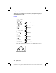
1. Press
z
. Select
Seq
and the defaults. Press
p
~
. Select
Time
FORMAT
and the defaults. Press
y
[
STAT PLOT
] and turn off all stat
plots.
2. Press
o
. Enter functions to describe the number of rabbits (
U
n
) and
the number of wolves (
V
n
) for
M = .05
,
K = .001
,
G = .0002
,
D = .03
. (
V
n
-
1
and
U
n
-
1
are
2nd
operations on the keyboard.)
U
n
=U
n
-
1
(1+.05
N
.001V
n
-
1
)
V
n
=V
n
-
1
(1+.0002U
n
-
1
N
.03)
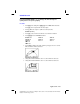
3. Press
p
and set the initial population of rabbits (
200
) and wolves
(
50
), the number of time periods to plot (
400
), and the size of the
viewing
WINDOW
.
U
n
Start = 200 Xmin = 0 Ymin = 0
V
n
Start = 50 Xmax = 400 Ymax = 300
n
Start = 0 Xscl = 100 Yscl = 100
n
Min = 0
n
Max = 400
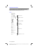
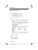
4. Press
r
to plot and explore the number of rabbits (
U
n
) and wolves
(
V
n
) over time (
n
). Determine the maximum and minimum number of
each.