Calculator User Manual

Chapter 9: Parametric Graphing
125
09PARA.DOC TI-86, Chap 9, US English Bob Fedorisko Revised: 02/13/01 2:27 PM Printed: 02/13/01 3:02 PM Page 125 of 809PARA.DOC TI-86, Chap 9, US English Bob Fedorisko Revised: 02/13/01 2:27 PM Printed: 02/13/01 3:02 PM Page 125 of 8

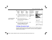
Enter these window variable values.
tMin=0 xMin=
L
20 yMin=
L
5
tMax=5 xMax=100 yMax=15
tStep=.1 xScl=50 yScl=10
- f
0
#
5
#
`
1
# a
20
#
100
#
50
# a
5
#
15
#
10

Set
SimulG
and
AxesOff
graphing formats,
so the path of the ball and the vectors will
be plotted simultaneously on a clear graph
screen.
/ ( # # #
" b # # "
b

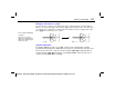
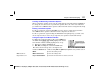
Plot the graph. The plotting action
simultaneously shows the ball in flight and
the vertical and horizontal component
vectors of the motion.
*

Trace the graph to obtain numerical results.
Tracing begins at
tMin
and traces the path
of the ball over time. The value displayed
for
x
is distance;
y
is height;
t
is time.
) "
Defining a Parametric Graph
The steps for defining a parametric graph are similar to the steps for defining a function
graph. This chapter assumes that you are familiar with Chapter 5: Function Graphing and
Chapter 6: Graph Tools. This chapter details those aspects of parametric graphing that
differ from function graphing.
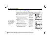
To simulate the ball in flight,
change the graph style of
xt1
à
yt1
to
Á
(animate).