Calculator User Manual

140
Chapter 10: Differential Equation Graphing
10DIFFEQ.DOC TI-86, Chap 10, US English Bob Fedorisko Revised: 02/13/01 2:28 PM Printed: 02/13/01 3:02 PM Page 140 of 2010DIFFEQ.DOC TI-86, Chap 10, US English Bob Fedorisko Revised: 02/13/01 2:28 PM Printed: 02/13/01 3:02 PM Page 140 of 2010DIFFEQ.DOC TI-86, Chap 10, US English Bob Fedorisko Revised: 02/13/01 2:28 PM Printed: 02/13/01 3:02 PM Page 140 of 20

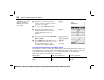
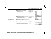
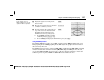
Display the axes editor and enter the
equation variable for which you want to
solve. (Do not set
y=Q
.)

Accept or change
fldRes
(resolution).
) &
1

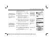
Display the graph. With the default
window variable values set, the slope
fields for this graph are not very
illustrative.
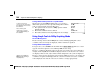
- i

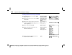
Change the window variables
xMin
,
xMax
,
yMin
, and
yMax
.

Select
TRACE
from the
GRAPH
menu to re-
plot the graph and activate the trace cursor.
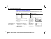
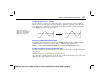
Trace the solution. The trace cursor
coordinates for
t
and
Q1
are displayed.
' # # # #
0
#
5
# #
0
#
20
/ )
" and !
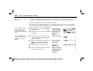
Transforming an Equation into a First-Order System
On the TI
-
86, to enter a second-order or higher (up to ninth-order) differential equation, you
must transform it to a system of first-order differential equations. For example, to enter the
second-order differential equation y''=
L
y, you must transform it to two first-order
differential equations, as shown in the chart below.
Differentiate... Define the variables as... And then substitute:
Q'1
=y'
Q1
=y
Q'1=Q2
(since
Q'1
=y'=
Q2
)
Q'2
=y''
Q2
=y'
Q'2=
L
Q1
In
SlpFld
field format,
x=t
is
always true;
y=Q1
and
fldRes=15
are the default
axes settings.