
Owner's Manual
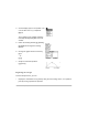
Table Of Contents
- Getting Started
- Initial start-up
- TI-89 Titanium keys
- Mode settings
- Using the Catalog to access commands
- Calculator Home screen
- Working with Apps
- Checking status information
- Turning off the Apps desktop
- Using the clock
- Using menus
- Using split screens
- Managing Apps and operating system (OS) versions
- Connecting your TI-89 Titanium to other devices
- Batteries
- Previews
- Performing Computations
- Showing Computations
- Finding the Factorial of Numbers
- Expanding Complex Numbers
- Finding Prime Factors
- Finding Roots
- Expanding Expressions
- Reducing Expressions
- Factoring Polynomials
- Solving Equations
- Solving Equations with a Domain Constraint
- Solving Inequalities
- Finding the Derivative of Functions
- Finding Implicit Derivatives
- Converting Angle Measures
- Symbolic Manipulation
- Constants and Measurement Units
- Basic Function Graphing I
- Basic Function Graphing II
- Basic Function Graphing III
- Parametric Graphing
- Polar Graphing
- Sequence Graphing
- 3D Graphing
- Differential Equation Graphing
- Additional Graphing Topics
- Tables
- Split Screens
- Data/Matrix Editor
- Statistics and Data Plots
- Programming
- Text Operations
- Numeric Solver
- Number Bases
- Memory and Variable Management
- Performing Computations
- Operating the Calculator
- Turning the Calculator On and Off
- Setting the Display Contrast
- The TI-89 Titanium Keyboard
- Modifier Keys
- Entering Alphabetic Characters
- Entering Numbers
- Entering Expressions and Instructions
- Formats of Displayed Results
- Editing an Expression in the Entry Line
- Menus
- Selecting an Application
- Setting Modes
- Using the Clean Up Menu to Start a New Problem
- Using the Catalog Dialog Box
- Storing and Recalling Variable Values
- Status Line Indicators in the Display
- Calculator Home Screen
- Calculator Home Screen
- Saving the Calculator Home Screen Entries as a Text Editor Script
- Cutting, Copying, and Pasting Information
- Reusing a Previous Entry or the Last Answer
- Auto-Pasting an Entry or Answer from the History Area
- Creating and Evaluating User-Defined Functions
- If an Entry or Answer Is “Too Big”
- Using the Custom Menu
- Finding the Software Version and ID Number
- Symbolic Manipulation
- Using Undefined or Defined Variables
- Using Exact, Approximate, and Auto Modes
- Automatic Simplification
- Delayed Simplification for Certain Built-In Functions
- Substituting Values and Setting Constraints
- Overview of the Algebra Menu
- Common Algebraic Operations
- Overview of the Calc Menu
- Common Calculus Operations
- User-Defined Functions and Symbolic Manipulation
- If You Get an Out-of-Memory Error
- Special Constants Used in Symbolic Manipulation
- Constants and Measurement Units
- Entering Constants or Units
- Converting from One Unit to Another
- Setting the Default Units for Displayed Results
- Creating Your Own User-Defined Units
- List of Pre-Defined Constants and Units
- Defaults for SI and ENG/US
- Constants
- Length
- Area
- Volume
- Time
- Velocity
- Acceleration
- Temperature
- Luminous Intensity
- Amount of Substance
- Mass
- Force
- Energy
- Power
- Pressure
- Viscosity, Kinematic
- Viscosity, Dynamic
- Frequency
- Electric Current
- Charge
- Potential
- Resistance
- Conductance
- Capacitance
- Mag Field Strength
- Mag Flux Density
- Magnetic Flux
- Inductance
- Basic Function Graphing
- Overview of Steps in Graphing Functions
- Setting the Graph Mode
- Defining Functions for Graphing
- Selecting Functions to Graph
- Setting the Display Style for a Function
- Defining the Viewing Window
- Changing the Graph Format
- Graphing the Selected Functions
- Displaying Coordinates with the Free-Moving Cursor
- Tracing a Function
- Using Zooms to Explore a Graph
- Using Math Tools to Analyze Functions
- Overview of the Math Menu
- Finding y(x) at a Specified Point
- Finding a Zero, Minimum, or Maximum within an Interval
- Finding the Intersection of Two Functions within an Interval
- Finding the Derivative (Slope) at a Point
- Finding the Numerical Integral over an Interval
- Finding an Inflection Point within an Interval
- Finding the Distance between Two Points
- Drawing a Tangent Line
- Finding an Arc Length
- Shading the Area between a Function and the x Axis
- Shading the Area between Two Functions within an Interval
- Polar Graphing
- Parametric Graphing
- Sequence Graphing
- 3D Graphing
- Overview of Steps in Graphing 3D Equations
- Differences in 3D and Function Graphing
- Moving the Cursor in 3D
- Rotating and/or Elevating the Viewing Angle
- Animating a 3D Graph Interactively
- Changing the Axes and Style Formats
- Contour Plots
- Example: Contours of a Complex Modulus Surface
- Implicit Plots
- Example: Implicit Plot of a More Complicated Equation
- Differential Equation Graphing
- Overview of Steps in Graphing Differential Equations
- Differences in Diff Equations and Function Graphing
- Setting the Initial Conditions
- Defining a System for Higher-Order Equations
- Example of a 2nd-Order Equation
- Example of a 3rd-Order Equation
- Setting Axes for Time or Custom Plots
- Example of Time and Custom Axes
- Example Comparison of RK and Euler
- Example of the deSolve( ) Function
- Troubleshooting with the Fields Graph Format
- Tables
- Additional Graphing Topics
- Collecting Data Points from a Graph
- Graphing a Function Defined on the Home Screen
- Graphing a Piecewise Defined Function
- Graphing a Family of Curves
- Using the Two-Graph Mode
- Drawing a Function or Inverse on a Graph
- Drawing a Line, Circle, or Text Label on a Graph
- Clearing All Drawings
- Drawing a Point or a Freehand Line
- Erasing Individual Parts of a Drawing Object
- Drawing a Line Between Two Points
- Drawing a Circle
- Drawing a Horizontal or Vertical Line
- Drawing a Tangent Line
- Drawing a Line Based on a Point and a Slope
- Typing Text Labels
- From the Home Screen or a Program
- Saving and Opening a Picture of a Graph
- Animating a Series of Graph Pictures
- Saving and Opening a Graph Database
- Split Screens
- Data/Matrix Editor
- Statistics and Data Plots
- Overview of Steps in Statistical Analysis
- Performing a Statistical Calculation
- Statistical Calculation Types
- Statistical Variables
- Defining a Statistical Plot
- Statistical Plot Types
- Using the Y= Editor with Stat Plots
- Graphing and Tracing a Defined Stat Plot
- Using Frequencies and Categories
- If You Have a CBL 2™ or CBR™
- Programming
- Running an Existing Program
- Starting a Program Editor Session
- Overview of Entering a Program
- Overview of Entering a Function
- Calling One Program from Another
- Using Variables in a Program
- Using Local Variables in Functions or Programs
- String Operations
- Conditional Tests
- Using If, Lbl, and Goto to Control Program Flow
- Using Loops to Repeat a Group of Commands
- Configuring the TI-89 Titanium
- Getting Input from the User and Displaying Output
- Creating a Custom Menu
- Creating a Table or Graph
- Drawing on the Graph Screen
- Accessing Another TI-89 Titanium, a CBL 2, or a CBR
- Debugging Programs and Handling Errors
- Example: Using Alternative Approaches
- Assembly-Language Programs
- Text Editor
- Numeric Solver
- Number Bases
- Memory and Variable Management
- Checking and Resetting Memory
- Displaying the VAR-LINK Screen
- Displaying Information about Variables on the Home Screen
- Manipulating Variables and Folders with VAR-LINK
- Showing the Contents of a Variable
- Selecting Items from the List
- Folders and Variables
- Creating a Folder from the VAR-LINK Screen
- Creating a Folder from the Home Screen
- Setting the Current Folder from the Home Screen
- Setting the Current Folder from the MODE Dialog Box
- Renaming Variables or Folders
- Using Variables in Different Folders
- Listing Only a Specified Folder and/or Variable Type, or Flash application
- Copying or Moving Variables from One Folder to Another
- Locking or Unlocking Variables Folders, or Flash Applications
- Deleting a Folder from the VAR-LINK Screen
- Deleting a Variable or a Folder from the Home Screen
- Pasting a Variable Name to an Application
- Archiving and Unarchiving a Variable
- If a Garbage Collection Message Is Displayed
- Memory Error When Accessing an Archived Variable
- Connectivity
- Connecting Two Units
- Transmitting Variables, Flash Applications, and Folders
- Transmitting Variables under Program Control
- Upgrading the Operating System (OS)
- Important Operating System Download Information
- Backing Up Your Unit Before an Operating System Installation
- Where to Get Operating System Upgrades
- Transferring the Operating System
- Important:
- Do Not Attempt to Cancel an Operating System Transfer
- If You are Upgrading the Operating System on Multiple Units
- Error Messages
- Collecting and Transmitting ID Lists
- Compatibility among the TI-89 Titanium, Voyage™ 200, TI-89, and TI-92 Plus
- Activities
- Analyzing the Pole-Corner Problem
- Deriving the Quadratic Formula
- Exploring a Matrix
- Exploring cos(x) = sin(x)
- Finding Minimum Surface Area of a Parallelepiped
- Running a Tutorial Script Using the Text Editor
- Decomposing a Rational Function
- Studying Statistics: Filtering Data by Categories
- CBL 2™ Program for the TI-89 Titanium
- Studying the Flight of a Hit Baseball
- Visualizing Complex Zeros of a Cubic Polynomial
- Solving a Standard Annuity Problem
- Computing the Time-Value-of-Money
- Finding Rational, Real, and Complex Factors
- Simulation of Sampling without Replacement
- Using Vectors to Determine Velocity
- Symbols
- Numerics
- A
- B
- C
- D
- E
- F
- G
- H
- I
- K
- L
- M
- N
- O
- P
- Q
- R
- S
- T
- U
- V
- W
- X
- Y
- Z

Parametric Graphing 348
Be careful when using implied multiplication with t. For example:
Note: When using t, be sure implied multiplication is valid for your situation. You can use
the
Define command from the Home screen (see the Technical Reference module) to
define functions and equations for any graphing mode, regardless of the current mode.
The Y= Editor maintains an independent function list for each
Graph mode setting. For
example, suppose:
• In FUNCTION graphing mode, you define a set of
y(x) functions. You change to
PARAMETRIC graphing mode and define a set of x and y components.
• When you return to FUNCTION graphing mode, your
y(x) functions are still defined
in the Y= Editor. When you return to PARAMETRIC graphing mode, your x and y
components are still defined.
Selecting Parametric Equations
Selecting Parametric EquationsSelecting Parametric Equations
Selecting Parametric Equations
To graph a parametric equation, select either its x or y component or both. When you
enter or edit a component, it is selected automatically.
Selecting x and y components separately can be useful for tables as described in Tables.
With multiple parametric equations, you can select and compare all the x components or
all the y components.
Enter: Instead of: Because:
t
ùcos(60)
tcos(60) tcos is interpreted as a user-defined function
called tcos, not as implied multiplication.
In most cases, this refers to a nonexistent
function. So the TI-89 Titanium simply returns
the function name, not a number.