
Owner's Manual
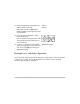

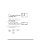
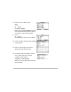
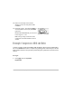
Table Of Contents
- Getting Started
- Initial start-up
- TI-89 Titanium keys
- Mode settings
- Using the Catalog to access commands
- Calculator Home screen
- Working with Apps
- Checking status information
- Turning off the Apps desktop
- Using the clock
- Using menus
- Using split screens
- Managing Apps and operating system (OS) versions
- Connecting your TI-89 Titanium to other devices
- Batteries
- Previews
- Performing Computations
- Showing Computations
- Finding the Factorial of Numbers
- Expanding Complex Numbers
- Finding Prime Factors
- Finding Roots
- Expanding Expressions
- Reducing Expressions
- Factoring Polynomials
- Solving Equations
- Solving Equations with a Domain Constraint
- Solving Inequalities
- Finding the Derivative of Functions
- Finding Implicit Derivatives
- Converting Angle Measures
- Symbolic Manipulation
- Constants and Measurement Units
- Basic Function Graphing I
- Basic Function Graphing II
- Basic Function Graphing III
- Parametric Graphing
- Polar Graphing
- Sequence Graphing
- 3D Graphing
- Differential Equation Graphing
- Additional Graphing Topics
- Tables
- Split Screens
- Data/Matrix Editor
- Statistics and Data Plots
- Programming
- Text Operations
- Numeric Solver
- Number Bases
- Memory and Variable Management
- Performing Computations
- Operating the Calculator
- Turning the Calculator On and Off
- Setting the Display Contrast
- The TI-89 Titanium Keyboard
- Modifier Keys
- Entering Alphabetic Characters
- Entering Numbers
- Entering Expressions and Instructions
- Formats of Displayed Results
- Editing an Expression in the Entry Line
- Menus
- Selecting an Application
- Setting Modes
- Using the Clean Up Menu to Start a New Problem
- Using the Catalog Dialog Box
- Storing and Recalling Variable Values
- Status Line Indicators in the Display
- Calculator Home Screen
- Calculator Home Screen
- Saving the Calculator Home Screen Entries as a Text Editor Script
- Cutting, Copying, and Pasting Information
- Reusing a Previous Entry or the Last Answer
- Auto-Pasting an Entry or Answer from the History Area
- Creating and Evaluating User-Defined Functions
- If an Entry or Answer Is “Too Big”
- Using the Custom Menu
- Finding the Software Version and ID Number
- Symbolic Manipulation
- Using Undefined or Defined Variables
- Using Exact, Approximate, and Auto Modes
- Automatic Simplification
- Delayed Simplification for Certain Built-In Functions
- Substituting Values and Setting Constraints
- Overview of the Algebra Menu
- Common Algebraic Operations
- Overview of the Calc Menu
- Common Calculus Operations
- User-Defined Functions and Symbolic Manipulation
- If You Get an Out-of-Memory Error
- Special Constants Used in Symbolic Manipulation
- Constants and Measurement Units
- Entering Constants or Units
- Converting from One Unit to Another
- Setting the Default Units for Displayed Results
- Creating Your Own User-Defined Units
- List of Pre-Defined Constants and Units
- Defaults for SI and ENG/US
- Constants
- Length
- Area
- Volume
- Time
- Velocity
- Acceleration
- Temperature
- Luminous Intensity
- Amount of Substance
- Mass
- Force
- Energy
- Power
- Pressure
- Viscosity, Kinematic
- Viscosity, Dynamic
- Frequency
- Electric Current
- Charge
- Potential
- Resistance
- Conductance
- Capacitance
- Mag Field Strength
- Mag Flux Density
- Magnetic Flux
- Inductance
- Basic Function Graphing
- Overview of Steps in Graphing Functions
- Setting the Graph Mode
- Defining Functions for Graphing
- Selecting Functions to Graph
- Setting the Display Style for a Function
- Defining the Viewing Window
- Changing the Graph Format
- Graphing the Selected Functions
- Displaying Coordinates with the Free-Moving Cursor
- Tracing a Function
- Using Zooms to Explore a Graph
- Using Math Tools to Analyze Functions
- Overview of the Math Menu
- Finding y(x) at a Specified Point
- Finding a Zero, Minimum, or Maximum within an Interval
- Finding the Intersection of Two Functions within an Interval
- Finding the Derivative (Slope) at a Point
- Finding the Numerical Integral over an Interval
- Finding an Inflection Point within an Interval
- Finding the Distance between Two Points
- Drawing a Tangent Line
- Finding an Arc Length
- Shading the Area between a Function and the x Axis
- Shading the Area between Two Functions within an Interval
- Polar Graphing
- Parametric Graphing
- Sequence Graphing
- 3D Graphing
- Overview of Steps in Graphing 3D Equations
- Differences in 3D and Function Graphing
- Moving the Cursor in 3D
- Rotating and/or Elevating the Viewing Angle
- Animating a 3D Graph Interactively
- Changing the Axes and Style Formats
- Contour Plots
- Example: Contours of a Complex Modulus Surface
- Implicit Plots
- Example: Implicit Plot of a More Complicated Equation
- Differential Equation Graphing
- Overview of Steps in Graphing Differential Equations
- Differences in Diff Equations and Function Graphing
- Setting the Initial Conditions
- Defining a System for Higher-Order Equations
- Example of a 2nd-Order Equation
- Example of a 3rd-Order Equation
- Setting Axes for Time or Custom Plots
- Example of Time and Custom Axes
- Example Comparison of RK and Euler
- Example of the deSolve( ) Function
- Troubleshooting with the Fields Graph Format
- Tables
- Additional Graphing Topics
- Collecting Data Points from a Graph
- Graphing a Function Defined on the Home Screen
- Graphing a Piecewise Defined Function
- Graphing a Family of Curves
- Using the Two-Graph Mode
- Drawing a Function or Inverse on a Graph
- Drawing a Line, Circle, or Text Label on a Graph
- Clearing All Drawings
- Drawing a Point or a Freehand Line
- Erasing Individual Parts of a Drawing Object
- Drawing a Line Between Two Points
- Drawing a Circle
- Drawing a Horizontal or Vertical Line
- Drawing a Tangent Line
- Drawing a Line Based on a Point and a Slope
- Typing Text Labels
- From the Home Screen or a Program
- Saving and Opening a Picture of a Graph
- Animating a Series of Graph Pictures
- Saving and Opening a Graph Database
- Split Screens
- Data/Matrix Editor
- Statistics and Data Plots
- Overview of Steps in Statistical Analysis
- Performing a Statistical Calculation
- Statistical Calculation Types
- Statistical Variables
- Defining a Statistical Plot
- Statistical Plot Types
- Using the Y= Editor with Stat Plots
- Graphing and Tracing a Defined Stat Plot
- Using Frequencies and Categories
- If You Have a CBL 2™ or CBR™
- Programming
- Running an Existing Program
- Starting a Program Editor Session
- Overview of Entering a Program
- Overview of Entering a Function
- Calling One Program from Another
- Using Variables in a Program
- Using Local Variables in Functions or Programs
- String Operations
- Conditional Tests
- Using If, Lbl, and Goto to Control Program Flow
- Using Loops to Repeat a Group of Commands
- Configuring the TI-89 Titanium
- Getting Input from the User and Displaying Output
- Creating a Custom Menu
- Creating a Table or Graph
- Drawing on the Graph Screen
- Accessing Another TI-89 Titanium, a CBL 2, or a CBR
- Debugging Programs and Handling Errors
- Example: Using Alternative Approaches
- Assembly-Language Programs
- Text Editor
- Numeric Solver
- Number Bases
- Memory and Variable Management
- Checking and Resetting Memory
- Displaying the VAR-LINK Screen
- Displaying Information about Variables on the Home Screen
- Manipulating Variables and Folders with VAR-LINK
- Showing the Contents of a Variable
- Selecting Items from the List
- Folders and Variables
- Creating a Folder from the VAR-LINK Screen
- Creating a Folder from the Home Screen
- Setting the Current Folder from the Home Screen
- Setting the Current Folder from the MODE Dialog Box
- Renaming Variables or Folders
- Using Variables in Different Folders
- Listing Only a Specified Folder and/or Variable Type, or Flash application
- Copying or Moving Variables from One Folder to Another
- Locking or Unlocking Variables Folders, or Flash Applications
- Deleting a Folder from the VAR-LINK Screen
- Deleting a Variable or a Folder from the Home Screen
- Pasting a Variable Name to an Application
- Archiving and Unarchiving a Variable
- If a Garbage Collection Message Is Displayed
- Memory Error When Accessing an Archived Variable
- Connectivity
- Connecting Two Units
- Transmitting Variables, Flash Applications, and Folders
- Transmitting Variables under Program Control
- Upgrading the Operating System (OS)
- Important Operating System Download Information
- Backing Up Your Unit Before an Operating System Installation
- Where to Get Operating System Upgrades
- Transferring the Operating System
- Important:
- Do Not Attempt to Cancel an Operating System Transfer
- If You are Upgrading the Operating System on Multiple Units
- Error Messages
- Collecting and Transmitting ID Lists
- Compatibility among the TI-89 Titanium, Voyage™ 200, TI-89, and TI-92 Plus
- Activities
- Analyzing the Pole-Corner Problem
- Deriving the Quadratic Formula
- Exploring a Matrix
- Exploring cos(x) = sin(x)
- Finding Minimum Surface Area of a Parallelepiped
- Running a Tutorial Script Using the Text Editor
- Decomposing a Rational Function
- Studying Statistics: Filtering Data by Categories
- CBL 2™ Program for the TI-89 Titanium
- Studying the Flight of a Hit Baseball
- Visualizing Complex Zeros of a Cubic Polynomial
- Solving a Standard Annuity Problem
- Computing the Time-Value-of-Money
- Finding Rational, Real, and Complex Factors
- Simulation of Sampling without Replacement
- Using Vectors to Determine Velocity
- Symbols
- Numerics
- A
- B
- C
- D
- E
- F
- G
- H
- I
- K
- L
- M
- N
- O
- P
- Q
- R
- S
- T
- U
- V
- W
- X
- Y
- Z

Differential Equation Graphing 434
Predator-Prey Model
Predator-Prey ModelPredator-Prey Model
Predator-Prey Model
Use the two coupled 1st-order differential equations:
y1' = Ly1 + 0.1y1 ùy2 and y2' = 3y2 Ny1 ùy2
where:
y1 = Population of foxes
yi1 = Initial population of foxes (2)
y2 = Population of rabbits
yi2 = Initial population of rabbits (5)
1. Use 3 to set
Graph = DIFF
EQUATIONS
.
2. In the Y= Editor (8#), define the
differential equations and enter the
initial conditions.
Note: To speed up graphing times, clear
any other equations in the Y= Editor. With
FLDOFF, all equations are evaluated even
if they are not selected.
3. Press:
,
9
— or —
@8Í Set
Axes = ON, Labels = ON,
Solution Method = RK, and
Fields = FLDOFF.