Calculator User Manual

876 Appendix A: Functions and Instructions
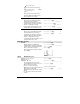
simult() MATH/Matrix menu
simult( coeffMatrix , constVector [, tol ]) ⇒
⇒⇒
⇒ matrix
Returns a column vector that contains the
solutions to a system of linear equations.
coeffMatrix must be a square matrix that contains
the coefficients of the equations.
constVector must have the same number of rows
(same dimension) as
coeffMatrix and contain the
constants.
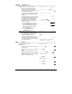
Optionally, any matrix element is treated as zero
if its absolute value is less than
tol . This tolerance
is used only if the matrix has floating-point
entries and does not contain any symbolic
variables that have not been assigned a value.
Otherwise,
tol is ignored.
• If you use ¥¸ or set the mode to
Exact/Approx=APPROXIMATE, computations
are done using floating-point arithmetic.
• If
tol is omitted or not used, the default
tolerance is calculated as:
5Eë 14 ù max(dim( coeffMatrix ))
ù rowNorm(
coeffMatrix )
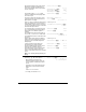
Solve for x and y: x + 2y = 1
3x + 4y =
ë 1
simult([1,2;3,4],[1;
ë1]) ¸
[
[[
[
ë 3
33
3
2
22
2
]
]]
]
The solution is x=
ë 3 and y=2.
Solve: ax + by = 1
cx + dy = 2
[a,b;c,d]
!matx1 ¸ [
a b
c d
]
simult(matx1,[1;2])
¸








ë (2ø bì d)
a
ø dì bø c
2
ø aì c
a
ø dì bø c
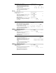
simult( coeffMatrix , constMatrix [, tol ]) ⇒
⇒⇒
⇒ matrix
Solves multiple systems of linear equations,
where each system has the same equation
coefficients but different constants.
Each column in
constMatrix must contain the
constants for a system of equations. Each column
in the resulting matrix contains the solution for
the corresponding system.
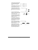
Solve: x + 2y = 1
3x + 4y =
ë 1
simult([1,2;3,4],[1,2;
ë1,ë3])
¸
[
ë 3 ë 7
2 9/2
]
For the first system, x=ë 3 and y=2. For the
second system, x=ë 7 and y=9/2.
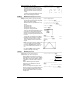
sin() 2W key
sin( expression1 ) ⇒
⇒⇒
⇒ expression
sin(
list1 ) ⇒
⇒⇒
⇒ list
sin(
expression1 ) returns the sine of the argument
as an expression.
sin( list1 ) returns a list of the sines of all elements
in
list1 .
Note: The argument is interpreted as a degree,
gradian or radian angle, according to the current
angle mode. You can use ó ,
G
or ô to override
the angle mode setting temporarily.
In Degree angle mode:
sin((p/4)ô ) ¸
‡2
2
sin(45)
¸
‡2
2
sin({0,60,90})
¸ {0
‡3
2
1}
In Gradian angle mode:
sin(50) ¸
‡2
2
In Radian angle mode:
sin(p/4) ¸
‡2
2
sin(45
¡) ¸
‡2
2