Technical data

Algorithm Optimization Examples
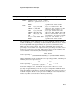
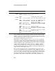
Example A–1 Core Loop of a BLAS 1 Routine Using Vector-Vector Operations
xAXPY - computes Y(I) = Y(I) + aX(I)
where x = precision = F, D, G
MSYNC ;synchronize with scalar
LOOP:
VLDx X(I),std,VR0 ;X(I) is loaded into VR0
VSMULx a,VR0,VR0 ;VR0 gets the product of VR0
;and the scalar value "a"
VLDx Y(I),std,VR1 ;Y(I) get loaded into VR1
VVADDx VR0,VR1,VR1 ;VR1 gets VR0 summed with VR1
VSTx VR1,Y(I),std ;VR1 is stored back into Y(I)
INC I ;increment I by vector length
IF (I < SIZ) GOTO LOOP ;Loop for all values of I
MSYNC ;synchronize with scalar
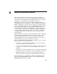
The performance of the Linpack 100 by 100 benchmark, which calls the
routine in Example 3–7 showing execution without chain into store, shows
how an algorithm with approximately 80 percent vectorization can be
limited by the scalar portion. One form of Amdahl’s Law relates the
percentage of vectorized code compared to the percentage of scalar code to
define an overall vector speedup. This ratio between scalar runtime and
vector runtime is described by the following formula:
Time Scalar
Vector Speedup = ______________________________________________
(%scalar*Time Scalar)) + (%vector*Time Vector)
Under Amdahl’s Law, the maximum vector speedup possible, assuming an
infinitely fast vector processor, is:
1.0 1.0
Vector Speedup = ____________________ = ____ = 5.0
(.2)*1.0 + (.8)*0 0.2
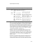
As shown in Figure A–1, the Model 400 processor achieves a vector
speedup of approximately 3 for the 100 by 100 Linpack benchmark when
using the BLAS 1 subroutines. It follows Amdahl’s Law closely because it
is small enough to fit the vector processor’s 1-Mbyte cache and, therefore,
incurs very little overhead due to memory hierarchy.
A–3