
Technical data

Algorithm Optimization Examples
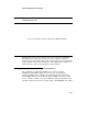
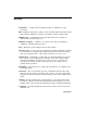
When the value of N is relatively small (that is, N < 256), the two-
dimensional FFT can be computed by calling a one-dimensional FFT of
length N**2. The small two-dimensional FFT can achieve performance
equal to that of the aggregate size one-dimensional FFT by linearizing the
data array. Figure A–7 shows the tradeoff between using the linearized
two-dimensional routine (for small N) and the transposed method (for
large N) to maintain high performance across all data sizes.
The optimization of an algorithm that vectorizes poorly in its original form
has been shown. The resulting algorithm yields much higher performance
on the VAX 6000 Model 400 processor. High performance is due to the
unique way the algorithm touches contiguous memory locations and its
effort to maximize the vector length. The implementation described above
always uses unity stride vectors and always results in a vector length of
64 for FFT lengths greater than 2K (2 x 1024).
Figure A–7 Two-Dimensional Fast Fourier Transform Performance Graph,
Optimized Single-Precision Complex Transforms
Refer to the printed version of this book, EK–60VAA–PG.
A–12