EE13 Updating Selected Laboratories for Engineering Experimentation Course at Worcester Polytechnic Institute A Major Qualifying Project Report Submitted to the Faculty of the WORCESTER POLYTECHNIC INSTITUTE in partial fulfillment of the requirements for the Degree of Bachelor of Science By _______________________ Mengjie Liu Date: April 25, 2012 _______________________________ Cosme Furlong, Advisor
Abstract This project aimed at updating two existing laboratories in Engineering Experiment course at Worcester Polytechnic Institute: Strain and Pressure Measurement Laboratory and Vibration Measurement Laboratory. Without major alternation to the experiment designs, the author examined laboratory equipment, software and instruction materials for both laboratories.
Acknowledgements I am grateful for all the help received during the process of this project. I thank my advisor Professor Cosme Furlong for making this project possible, and for all the valuable guidance and advices. I appreciate WPI Mechanical Engineering department for providing the experiment equipment, especially Lab Manager Peter Hefti for offering help and support in the lab, and past Teaching Assistant for Engineering Experimentation course Ivo Dobrev for providing helpful information.
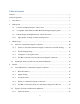
Table of Contents Abstract ........................................................................................................................................... 1 Acknowledgements ......................................................................................................................... 2 1. Introduction ............................................................................................................................. 1 2. Background .........................................
. 4.2.2 Updated Instruction Materials for Strain and Pressure Measurement Laboratory 25 4.2.3 Updated Instruction Materials for Vibration Measurement Laboratory ................ 25 Conclusions and Future Work .............................................................................................. 27 Works Cited ...................................................................................Error! Bookmark not defined.
Table of Tables Table 1 Parameters for Testing ..................................................................................................... 12 Table 2 Comparison of Signal Conditioners’ Basic Parameters ................................................... 16 Table 3 Shunt Resistor Testing Result for Signal Conditioners ................................................... 17 Table 4 Accuracy Test Result ...................................................................................................
Table of Figures Figure 1 System Schematic of Strain Measurement Set-up.......................................................... 10 Figure 2 DATAQ’s Signal Response to Shunt Resistor ............................................................... 18 Figure 3 Connections for Tacuna Systems Strain Gauge or Load Cell Amplifier/Conditioner Interface Manual ...........................................................................................................................
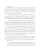
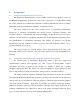
1. Introduction ABET accreditation criteria requires undergraduate engineering programs to prepare students with “an ability to design and conduct experiments, as well as to analyze and interpret data”, and mechanical engineering curriculums to “require students to apply principles of engineering, basic science and mathematics”, and “prepare students to work professionally in both thermal and mechanical systems.
techniques involved. The equipment should enable acceptable level of accuracy and resolution. Student Experience. The instructive materials should prepare the students with relevant theoretical background, give clear and organized instructions that are easy to follow, and provide challenging questions and assignments. The equipment should be safe and easy to operate, and it should enable hands-on experience to deepen students’ understanding of the equipment’s operating principle.
2. Background 2.1 Contents and Implementation of the Course The Engineering Experimentation course at WPI is a junior-level compulsory course for the Mechanical Engineering program; the coursework is equivalent to 3 credits. Before taking this course, students are recommended to finish the compulsory fundamental courses in ordinary differential equations, thermal-fluid, mechanics, and material science.
Familiarity of computerized data acquisition system is cultivated in required courses in the majority of programs investigated, and a significant amount of programs teaches the use of traditional tools such as oscilloscope and function generator. Other frequently taught topics include frequency response and Fourier transformation, experiments in fluid mechanics, and material testing.
acquire data in strains as the Strain and Pressure Measurement Laboratory, including strain gauges, a Wheatstone bridge, a signal conditioning system, and an analog/digital converter. 2.2.2 Opportunities for Improvements and Expansions Laboratories that measures pressure and vibration with strain gauges are frequently taught at colleges.
temperature and pressure vary, which unsettles the equilibrium of fluids and carbon dioxide in the can. For these stated sources or variability, the students can gain more insights of the experiment from a relatively large amount of measurements. Therefore, use of a “class data sheet” to gather experiment results can be beneficial.
error in finding the “effective length” adds uncertainty to the elastic modulus estimation. The boundary condition created by the fixture made of a c-clamp and the lab bench makes the set-up slightly deviates from the simple cantilever model. The issue can be alleviated by simply adding a piece of aluminum plate between the clamp and the beam. A special fixture tool with a rectangle shape that rigidly clamps the beam can provide the ideal boundary condition.
Finite Element simulation (Kargar, S; Bardot, D.M. ., 2010) to simplified method of drawing a smooth curve to connect the data points on a plot with distance from the hole against the local strain (Stress and Strain Concentration, 2003).
2.2.2.5 Software The course requires no previous experience of programming in LabVIEW, therefore, the instructive materials need to guide the students to construct simple functional programs to facilitate the experiment. More advanced LabVIEW programs can be provided to the students to use in the laboratories. Some of the suitable features to add to the basic programs are: filters, data processing, and data reporting.
3. Methodology 3.1 Selection of Alternative Signal Conditioners 3.1.1 Selection of Potential Alternative Signal Conditioners for In-Lab Testing The two target laboratories, strain and pressure measurement laboratory, and vibration measurement laboratory, use the same set up for strain measurement. The hardware set-up includes a signal conditioner unit that supplies excitation voltage and amplifies output signal from the Wheatstone bridge.
In the case of the current set-up, the range can be set to 5V. Thus, the resolution is 0.22mV. Amplifier gain determines the transfer function between signal voltage and represented strain. When gain is 200, the resolution represents 0.23 microstrain. In order to enable successful implementation of the laboratories, suitable signal conditioners should satisfy a series of requirements.
Vishay Omega Honeywell DATAQ 2310 DMD-465WB UV-10 DI5B38-04 Excitation 10V 10V 5V 10V 5V Gain 191 239* 200 333.3 220 Warm-up Time 0 45 min 10 min 10 min 5 min Tacuna Table 1 Parameters for Testing Strain load can be simulated when a shunt resistor is connected to the Wheatstone bridge in parallel to the active gauge. For the first output testing, three different shunt resistors are used to simulate three different strains for each signal conditioner.
The Error is the percentage difference between measured strain and simulated strain. The Maximum Error is the largest observed error in the five samples taken. The Average Error is given by: ̅ where √ is the Error of each reading. For each reading, the standard deviation of the signals after applying simulated load is calculated; this is equivalent to RMS noise. Peak-to-peak noise amplitude is within 8 times RMS value 98% of the time.
3.1.4 Test Run of the Laboratories with Selected Signal Conditioners Test run of the laboratories are performed with selected signal conditioners for further validation. Sample laboratory reports are generated for reference. 3.2 Updating Software and Laboratory Instruction Materials The current VIs is examined. Improvements are made to the program for usability, without any major alternation of the program design. Detailed step-by-step tutorial for constructing these VIs are written.
4. Results This project recommended two alternative signal conditioners for use in Strain and Pressure Measurement Laboratory and Vibration Measurement Laboratory, and updated the LabVIEW programs and instruction materials for both laboratories. 4.
Vishay Omega Honeywell DATAQ 2310 DMD-465WB UV-10 DI5B38-041 115VAC 115VAC 18 - 32 VDC 5VDC 6-16VDC Excitation 0.5-15 VDC, 4 to 15VDC 3, 5 and 10 V, Voltage 12 settings Manual adjust Manual adjust 10VDC 5VDC Max 100 mA Max 120mA Max 70mA 70-170mA Max 100 mA Automatic N/A Manual N/A Manual 1-11000 40–250, continuous manual adjust 333.
4.1.2 Output Testing With the method described in section 3.1.2 of this report, the noise, accuracy, and precision of measurements are evaluated. Table 3 shows the analysis results when the strains are simulated with shunt resistors. Vishay Omega Honeywell DATAQ 2310 DMD-465WB UV-10 DI5B38-04 0.24 2.46 2.14 4.99 0.18 0.24 3.94 4.09 11.44 0.31 1.93 19.71 16.8 39.95 1.44 1.93 31.49 32.7 91.54 2.48 Maximum Error 2.6% 9.3% 2.9% 12.5% 3.5% Average Error 1.7% 7.1% 1.7% 9.
Amplifiied Signal (V) 1 0.5 0 -0.5 0 5 10 Time (s) 15 20 25 Figure 2 DATAQ’s Signal Response to Shunt Resistor With the method described in section 3.1.2 of this report, the noise, accuracy, and are evaluated with actual strain of known values. Table 4 and Table 5 show the analysis results. Applied Load Omega Honeywell (micro strain) DMD-465WB UV-10 266.8 265.7 258.9 259.6 240.5 234.9 225.3 234 213.7 209.8 207.9 208.7 Error 2% 4% 2.
As shown in the test results, the current system, Vishay 2310, outperforms all other system in all measured aspects. It is, however, significantly higher cost than all other systems considered. The measured performance metrics for the four considered amplifier are ranked from 1 to 4, 1 being the best performance and 4 being the worst. As shown in Table 6, DATAQ DI5B38 shows the lowest performance compared to other systems, and therefore should be eliminated from the selection.
Figure 4 Location of Gain select switch and offset potentiometer G0 ON G1 OFF G2 OFF Table 7 Switch settings for Tacuna for 220 Gain 3. Bridge Balance Use the offset potentiometer to adjust the output voltage to 2.5V, which is half of the output range. It is required to open the enclosure to adjust the gain switches but not the offset potentiometer. The wire connections are located outside of the enclosure. 4.1.3.2 Set-up Procedure for Honeywell UV-10 1.
Figure 5 Connections for Honeywell UV-10 In-line Amplifier 2. Gain setting While excitation jumper is set to 5V, in order to get a gain of 200, make sure switch 3 and switch 6 are on and other switches are off. 3. Calibration With zero loads on the strain gauge, adjust the ZERO potentiometers until the reading approaches 0. It is required to open the enclosure to adjust both the ZERO potentiometers and the gain. The wire connections are located inside the enclosure as well. 4.1.3.
Figure 6 Connections for Omega DMD 465-WB 2. Set excitation voltage Connect a multi-meter to terminal 2 and 4; adjust potentiometer B+ until the reading approaches the desired excitation voltage. 3. Calibrate for zero voltage Jumper pin 8 and 9 together, connect the inputs of DAQ box to pin 11 and 10. Adjust the COARSE OFFSET and the FINE OFFSET potentiometers until the voltage approaches 0.
4. Adjust gain Connect the shunt resistor simulating strain desired for full scale. Adjust the COARSE GAIN and FINE gain potentiometers for the desired full scale output. All wire connections and potentiometers of this equipment are located on the surface of the enclosure. No discrete gain setting is available, or any gain indications. 4.1.3.
4.1.4 Selection of Alternative Signal Conditioner Tacuna Systems Strain Gauge or Load Cell Amplifier/Conditioner Interface Manual (Tacuna) provides reliable and quiet reading, and easy set-up experience. It is most viable economical alternative to currently used signal conditioner. Honeywell UV-10 In-line Amplifier provides satisfying performances as well, and a setup experience slightly more complex than Tacuna.
Node requires dynamic data to be converted to numerical data. This enables the program to process and record all acquired data points. The updated VI allows the user to input excitation voltage, gain, and gage factor; thus the program can be used with different hardware conditions without major alternation. Updated software for Vibration Measurement Laboratory enables saving time domain data without alternating the program.
o Mode shapes of a cantilever beam under free vibration o Damping factor of a cantilever beam under free vibration Measurement methods of dynamic characteristics o Fourier transformation o Logarithmic decrement method to determine damping frequency o Determining acceleration, velocity and amplitude o Determining elastic modulus Strain gages o Operating principle and application of strain gages o Materials and selection of strain gauges Wheatstone bridge The instructions describe the
5. Conclusions and Future Work This project examined two existing laboratories in WPI’s Engineering Experiment course and made a series of recommendations and actions, in the hope of improving the educational value, student experience and the cost-effectiveness of the laboratories. The project recommended two alternative signal conditioners to use in the laboratories. Both signal conditioners provide satisfactory performance and student experience, in addition to being economical.
Works Cited Poisson's Ratio. (2003). Retrieved December 2012, from Fulton School of Engineering, Arizona State University: http://enpub.fulton.asu.edu/imtl/HTML/Manuals/MC102_Poisson's_Ratio.html Stress and Strain Concentration. (2003). Retrieved Febuary 2013, from Fulton School of Engineeing, Arizona State University: http://enpub.fulton.asu.edu/imtl/HTML/Manuals/MC104_Stress_Concentration.htm ABET. (2012). Criteria for Accrediting Engineering Programs, 2012 - 2013 .
Mostic, K. (1990). Lab: Calibration of and Measurement with Strain Gages. Retrieved Dec 2012, from Northen Illinois University: http://www.kostic.niu.edu/Strain_gages.html Omega. (n.d.). User's Guide. Retrieved from Omega: http://www.omega.com/manuals/manualpdf/M1429.pdf Pryputniewicz, R. (1993). Notes: Engineering Experiementation. WPI. Ruff, J. (n.d.). Lab 6: Stress Concentration. Retrieved 2012, from New Mexico Tech: http://infohost.nmt.edu/~jruff/Lab6.pdf Tacuna Systems. (n.d.).
Appendix 1: Sample Laboratory Report for Strain and Pressure Measurement Laboratory Abstract In this experiment, characterization of internal pressure in a thin-walled tank (a soda can) is achieved by measurements of mechanical strains. Uncertainty analysis of characterized internal pressure is conducted with respect to parameters involved. The percentage contribution of all uncertainties to the overall uncertainty in pressure characterizations are identified in order of importance.
Experimental Procedures In order to understand the errors in this experiment, the procedure is repeated on three soda cans of the same product. Preparation Find the Poisson’s ratio and elastic modulus of the material used for the soda cans. LabVIEW Program The constructed LabVIEW program obtains amplified voltage output and transfers the output to strain, with the unit of micro-strain. A formula block calculates pressure and stress from measured strains. Measurement results are recorded. Assume 0.
Bridge Balancing and Verification Make sure then NI DAQ box is turned on before starting the VI. Adjust the measurement time to 0.01 second on the LabVIEW program to view instant strain readings. Use the offset potentiometer to adjust the output voltage to 2.5V, which is half of the output range. Connect shunt resistors parallel to the active gauge, and observe appropriate change in the strain reading. Gently press on the tap of the can, and observe the strain readings change accordingly.
Key Equations The expression for internal pressure of a thin-wall vessel can be given by: where E is Elastic Modulus of the material, is the Poisson’s ratio of the material, t is the wall thickness of the vessel, r is the radius of the vessel, is the strain in hoop (circumferential) direction. The stress in circumferential direction and axial direction is given by: where P is internal pressure of the vessel, r is the radius, and t is the wall thickness.
Results and Conclusions The results of the characterization are listed in Table 1. The parameters are calculated by taking the differences of the average values prior to opening of the cans and the average values after opening the cans. Can 1 (Fanta 355ml) Can 2 (Fanta 355ml) Can 3 (Fanta 355ml) Pressure Hoop Strain Hoop Stress Axial Stress (psi) (micro-strain) (psi) (psi) 35.0 750 43.7 937 48.
Uncertainty Analysis The parameters in Table 2 are used to perform uncertainty analysis for characterized internal pressure. The detailed process of the analysis is included in the appendix. Parameter Young's Modulus (psi) Poisson's Ratio Thickness (in) Radius (in) Strain (micro strain) Value Uncertainty 0.35 0.005 1.300 0.005 3% Table 2 Initial Parameters for Uncertainty Analysis The uncertainty for measured pressure is constant at 10.4% when strain is within the specified range.
Supplemental Materials LabVIEW Programming Figure 8 Front Panel of LabVIEW Program Figure 9 Block Diagram of LabVIEW Program 36
Uncertainty Analysis 37
38
39
40
Appendix 2: Sample Laboratory Report for Strain and Pressure Measurement Laboratory Abstract In this experiment, strain gauges are used to measure the dynamic characteristic and the material properties of cantilevers. The vibration data is analyzed to determine the parameters; the values derived from measurements are then compared with theoretical values and/or computational models.
Description Purpose of the Experiment The purpose of the vibration measurement experiment is to use strain gauges to measure the dynamic characteristic and the elastic material properties of cantilevers.
Experimental Procedures In order to understand the errors in this experiment, the procedure is repeated on two similar cantilever beams. Preparation Find the elastic modulus and density of the material used for the cantilever beams. LabVIEW Program The constructed LabVIEW program obtains amplified voltage output and transfers the output to strain, with the unit of micro-strain. A spectral analyzer performs Fourier Transformation on measured strains.
Bridge Balancing and Verification Make sure then NI DAQ box is turned on before starting the VI. Adjust the measurement time to 0.01 second on the LabVIEW program to view instant strain readings. Use the offset potentiometer to adjust the output voltage to 2.5V, which is half of the output range. Connect shunt resistors parallel to the active gauge, and observe appropriate change in the strain reading. Gently press on the tap of the can, and observe the strain readings change accordingly.
Key Equations Strain in a Cantilever under Known Load The strain in a cantilever beam under a known load applied at the free end is given by: where is the strain, P is the applied load, L is the length of the beam, x is the distance between the clamped end and the interested location of strain, E is the elastic modulus, b is the width of the beam, and T is the thickness of the beam. In this experiment, the applied load is the weight of a known mass.
The altitude is equivalent to maximum deflection at vibration peaks. The amplitude can be given by: Therefore, the maximum velocity and maximum acceleration can be expressed as: Damping Ratio A common method for analyzing the damping of an underdamped oscillation is the logarithmic decrement method, for which the following relationships apply.
Equipment List National Instruments USB-6229 DAQ Tacuna Systems Strain Gauge or Load Cell Amplifier/Conditioner Interface Manual Wheatstone Bridge Quarter Bridge Completion Circuit Vishay Strain Gage Shunt Resistors Three Cans of Soda of The Same Type A Cantilever Beam 47
Results and Conclusions Initial Measurements and Research The beams used in this experiment are made with 6061 Aluminum. The Modulus of Elasticity and density of the material are listed in Table 1. Parameter Value (SI Unit) Value (English Unit) 68.9GPa Young’s Modulus (E) 0.0975 lb/in³ Density (𝜌) Table 1 Material Property of 6061 Aluminum The measured beam dimensions and the gauge location for the beam is listed in Table 2.
Verification of Correct Installation To verify the correct installation, a weight attached close to the free end on the beam. The analytical strain at strain gauge location is derived and compared with measured values, as shown in Table 3. The error is within 3% compared to the theoretical strain derived, therefore, the installation is correct. Theoretical Strain Measured Strain (micro strain) (micro strain) 240.5 235 Error 2.
Theoretical Natural Measured Natural Frequency (Hz) Frequency (Hz) 35.5 35.3 Table 4 Comparison of Measured Fundamental Frequency and Theoretical Fundamental Frequency Determine the Vibration Amplitude, Velocity, and Acceleration Figure 2 shows the plot for the strain measured from one of the beams during free vibration. Strain (micro strain) 200 100 0 -100 -200 2.9 3.4 3.
Acceleration Acceleration Velocity Amplitude (m/s) (m) (g) Peak 6.6 64.7 1.84 0.052 Peak-To-Peak 13.2 129.4 3.67 0.104 RMS 4.7 45.8 1.30 0.036 Table 5 Maximum Acceleration, Velocity and Displacement Measure and Express Damping Characteristics Using logarithmic decrement method, the damping ratio for the beam is determined from measured data, as shown in Table 7. Logarithmic Decrement Damping Ratio 0.042 0.0067 Table 6 Damping Ratio Predict Elastic Modulus.
Uncertainty Analysis The uncertainty of natural frequency is 0.05 Hz, which is limited by the resolution of spectral analyzer in LabVIEW program. Uncertainty analyses with respect to the parameters are performed for damping ratio and amplitude. Parameters used in the uncertainty analyses are shown in Table 9. Thickness, length and gauge location are measured with a ruler, which has a least significant digit of Therefore, the uncertainty for these three items is inch, or inch. meter.
Supplemental Materials LabVIEW Program Figure 3 shows the front panel of the LabVIEW program used in this experiment. Figure 4 shows the block diagram of the LabVIEW program.
Uncertainty Analysis 54
55
56
57
58
Appendix 3: Instructions for Strain and Pressure Measurement Laboratory Laboratory: Strain and Pressure Measurement 1.
2. BACKGROUND A thin walled cylinder has a wall thickness smaller than 1/10 of the cylinder’s radius. In this case, only the membrane stresses are considered and the stresses are assumed to be constant throughout the wall thickness. The ASME boiler codes require continuous monitoring of pressure in thin walled pressure vessels.
Figure 1b Top View of a Pressure Transducer 2.2 Figure 1c Circuit Diagram of a Wheat Stone Bridge Stress and Strain in a Thin-Wall Cylinder For vessels with a wall thickness of no more than one-tenth of its radius, the wall can be treated as a surface. The law of LaPlace holds for fluid or gas filled hollow objects with radius r. For cylinders, the internal pressure acts on them to develop a force along the axis of the cylinder.
Similarly, in the axial direction, the pressure acts to push the two halves apart, while axial stress balances the effects, as shown in figure 3. The axial stress yields, Eq.3 Eq.4 The Hooke’s Law states that stress in the can is proportional to the strain. The relationship in this case can be expressed as: Eq.5 where E is Elastic Modulus of the material, and is Poisson’s ratio of the material. With Eq.2, Eq.4, and Eq.5, the relationship between pressure and strains can be derived as: Eq.6 2.
temperature, material properties, the adhesive that bonds the gage to the surface, and the stability of the metal. The strain sensitivity, which is also known as the gage factor (GF) of the sensor, is given by: Eq.8 where R is the resistance of the gauge without deformation, dR is the change in resistance caused by strain, and is the strain to be measured. Therefore, the strain can be expressed as: Eq.9 2.3.
Figure 17 Temperature Effects on Thermal Output of Strain Gauges Strain gauge’s product name contains all critical information needed to select appropriate gauge. The meanings of each part of the name are shown in Figure 18 below. While Figure 19 shows key information of the type of strain gauge selected for this experiment.
Figure 19 Crucial Information of Strain Gauge Selected 2.4 Basics of Wheatstone bridge A Wheatstone bridge is an electrical circuit used to measure an unknown electrical resistance (from 1 Ω to 1MΩ) by balancing two legs of a bridge circuit, one leg of which includes the unknown component. A circuit diagram of Wheatstone bridge is shown in figure below, where the battery (symbol “E” serves as an excitation source, and the output is measured by a potentiometer “G”).
Figure 6 circuit diagram of Wheatstone bridge When the bridge is unbalanced, equivalent resistance of the circuit is, Eq.10 When the circuit is viewed as a circuit divider, the output voltage is, ( When the resistance of ) ( Eq.11 ) changes by a small amount , the new output voltage is, Eq.12 ( If the bridge was originally balanced ( ( )( ) ) , then we have, Eq.13 ( Since change in resistance is really small ) , the change in output voltage is, or, Eq.
3. PROCEDURES In order to estimate the internal pressure of soda cans, the procedures of this experiment include research for relevant data, hardware set-up, construction of LabVIEW program, signal conditioning, taking measurements, and data analysis. The measurements should be repeated on 3 soda cans. The information acquired from research and part of the measurement process should also be used to produce uncertainty analysis and the contribution of each parameter to total uncertainty. 3.
To achieve an output signal of 1mV per , the gain (G) needs to satisfy: Therefore, Eq.17 For this experiment, gage factor (F) is 2.095 . 3.1.3 Calculate Strain Simulated by Shunt Resistors Calculate the strain simulated by shunt resistors. The connected shunt resistors are parallel to the gage, the equivalent resistance is: Eq.18 Therefore, Eq.19 Gage factor is 2.095 0.5% for the gauge chosen for this experiment. Resistance without deformation is 120 . 3.
Besides strain gauge and the cans, material needed for attaching the gauge to a surface include: sand paper, degreaser/alcohol, conditioner, neutralizer solutions, cotton balls & swabs, one-side sticky tape , adhesive , low-impedance strain gage wire (about 15 “) , and soldering material. The steps of are explained below. 1) Degreasing: wipe the surface with degreaser or alcohol to remove oil, grease, organic taminants and soluble chemical residues.
7) Lift tape: prior to applying adhesive, lift the end of tape opposite the solder tabs at a shallow angle, until the gauge and terminal is free from the surface. Tack the loose end of the tape under and press to the surface, so the gage lies flat with the bonding side exposed. Figure 21 Lift tape 8) Apply adhesive and attach: apply a drop of adhesive to the gage’s bonding side, attach the gauge and the surface by pressing on the tape for a minute.
11) Protecting the gage: apply a protective coating over the entire gage and terminal area. 12) Measure the base resistance of the unstrained strain gage after its proper mounting but before complete wiring. Check for surface contamination by measuring the isolation resistance between the gauge grid and the stressed force detector specimen by means of an ohmmeter, if the specimen is conductive. This should be done before connecting the lead wires to the instrumentation.
b. Enter relevant information into VI’s front panel, use standard thickness obtain from research as initial value. Press the can or slightly shake the can and observe the measured strains react as expected. Let the can settle (strains and pressure approach zero) before starting measurement. c. Run the VI for 10 seconds, then open the can, keep recording for another 10 to 20 seconds. Press “stop” button to make sure the data is recorded. Data will be saved in csv file in the same directory VI is saved.
4. DATA ANALYSIS & DISCUSSION With the results acquired with three soda cans, estimate the range of internal pressure of similar soda cans. Compare with the pressure value obtained through research. Conduct uncertainty analysis on the pressure measurements and Poisson’s ratio measurements. Assume 3% of uncertainty in strain measurements. Refer to provided sample uncertainty analysis.
Document 1: Soda Can Parameters and Uncertainty Estimation as a Reference a. Standard dimension of the soda can (diameter and thickness) and the uncertainties associated The standard values and factors contributing to uncertainty for can diameter and thickness of a soda can are listed in table below. 2 Standard Resolution Repeatability Standard Deviation (Assumed) (Assumed) Metric English Diameter 6.6 cm 2.6 in 0.001 in 0.005 in 0.0001in Thickness 0.013cm 0.005in 0.0001 in 0.
√ ( ) ( ) The beverage can lids are usually made from AA5182 H48, while bodies are usually made from AA 3004 or AA 3104 in the H 19 temper. This specification is sufficiently wide to permit suppliers to offer versions with higher formability or higher strength properties. Increase in material strength has been achieved by gradually increasing the magnesium content from the nominal 0.9% of 10 years ago, to nominal 1.1% today, and copper from nominal 0.06 to 0.15%.
c. Common internal pressure range of soda cans Gases exert a pressure on any surface with which they are in contact. The amount of pressure exerted by the molecules of a gas depends on the force and frequency of the molecules towards the walls of its container. The pressure of gases is therefore dependent upon temperature and volume. The Third Gas Law states that when the volume of a fixed mass of gas is maintained constant, pressure is directly proportional to absolute temperature.
Document 2: Set-Up Procedure for Signal Conditioner (Tacuna) a. Connection Connect the wires as indicated in Figure 1. Figure 1 Connections for Tacuna Systems Strain Gauge or Load Cell Amplifier/Conditioner Interface Manual b. Gain Setting To get a gain of 220, make sure the switches (location shown in Figure 4) are set as indicated in Table 1. Figure 23 Location of Gain select switch and offset potentiometer G0 ON G1 OFF G2 OFF Table 9 Switch settings for Tacuna for 220 Gain c.
It is required to open the enclosure to adjust the gain switches but not the offset potentiometer. The wire connections are located outside of the enclosure.
Document 3: Tutorial for LabVIEW Program This sample LabVIEW program for the Strain and Pressure Laboratory acquires the voltage input from connected NI DAQ device, calculates and indicates real-time strains experienced by the strain gauge, then calculates and saves dynamic values of internal pressure of the can, stress in both circumferential and axial directions of the can to a .csv file in the same folder where the LabVIEW program is saved, along with the micro strain readings.
80
On Front Panel, right click on a blank location and access the Controls Palette, under Express menu find Numeric Controls, then select a Num Ctrl by left clicking. The control can also be found through Search tool in the Controls Palette. After selecting the icon, move the pointer to desired location and left click to position the control on front panel. Then, click on the text above the control and edit the name of the control. In the same way, create all the numeric controls needed for this program.
Add Numeric Indicator and Waveform Graph for Micro Strain readings. The path for Numeric Indicator is Control Palette Express Numeric Indicators Numeric Indicator. The path for Waveform Graph is Control Palette Express Graph Indicators Graph.
Add a DAQ Assistant in the While Loop and configure the subVI with the wizard. (Functions Palette Measurement I/O NI DAQ mx DAQ Assistant). For the measurement type, select Acquire Signals Analog Input Voltage. For the physical channel, select the channel of incoming signal. Since channel AI0 of NI 6229 is connected to the input, select this specific channel. Next, configure the channel settings: input -10V to 10V for input signal range, and 1 Sample (On Demand) for acquisition mode.
On the block diagram, drag down the arrow on the bottom of the Formula icon to expand the input/output menu. To change the order of the elements, right click on an element and select “select input/output”, then click on the input/output desired for the position. Connect the data output of the DAQ Assistant, and the Numerical Controls for excitation voltage, gage factor and gain to the corresponding inputs of the Formula.
Calculated pressure, diameter and thickness are used to calculate circumferential stress and axial stress. The formulas are shown in the two figures below.
Dynamic data of micro strain, pressure, circumferential and axial stress are then combined with Merge Signal function and then written to file with a Write to Measurement File function. The merged signal should be connected to Signal Input of the Write to Measurement File function. The Filename can be constructed with Build Path function.
The Write to Measurement File should be configured as shown below. The filename in this wizard will be overwritten by the input; it should “save to one file”; the format should be text, with one header only or no headers; there should be only one time column; and the delimiter should be comma.
Now we have completed constructing the VI. If there is any error in the program, the run button will appear “broken” as shown in the figure below. Click on the button to view the error list, the “details” should explain the error. Debug until all errors are resolved; use other debugging functions on the menu bar if needed.
Document 4: Optional Activities in this Laboratory 1. Create a shared data file for the class; consolidate measured internal pressure from all the students. What is the average and standard deviation of the measured value? What are some of the possible causes of these variations? 2. Before opening the can in this experiment, shake the can for 5 seconds, measure the change in internal pressure. What are the possible causes of the change? 3.
Appendix 4: Instructions for Vibration Measurement Laboratory Laboratory: Vibration Measurements 1. OBJECTIVES This laboratory uses strain gauge to measure the dynamic characteristic and the elastic material properties of a cantilever.
2. BACKGROUND Health monitoring is the process of studying and assessing the integrity of structures, which is crucial for preventing failure and for achieving reliable designs. Health monitoring can be done by dynamic or static analysis, or a combination of both. In static analysis, deformations or changes in the orientation of structures, due to application of loads, or unexpected damages, are determined via comparisons with reference models.
maximum tensile force occurs at the upper most edge. The equation for determining the bending stress is Eq.1 where M is the applied moment, c is the distance from the neutral axis to the outer fiber of the beam, and I is the moment of inertia. The derivation of Eq.1 is shown in Appendix A. The maximum bending stress in a beam is Eq.2 where t is the thickness of the beam. Hooke’s law describes the relationship between stress and induced strains for linear elastic materials. Eq.
Figure 24 Neutral axis of a beam subjected to bending Euler—Bernoulli beam theory relates curvature of a bending beam to bending moment and rigidity of the material Eq.4 where E is the elastic modulus of the material, I is the second moment of area. I must be calculated with respect to the centroidal axis perpendicular to the applied loading. w is the deflection in distance, is the slope of the beam, and equals to the beam curvature , or .
distributed loads and uniformly varying loads over the span and a number of concentrated loads are conveniently handled using this technique. For general loadings, the bending moment M can be expressed in the form 〈 The quantity 〈 〈 〉 〈 〉 〈 〉 Eq.6 〉 is a Macaulay bracket, it is defined as 〉 { Eq.7 When integrating expressions containing Macaulay brackets, we have ∫ 〈 〉 〈 Eq.8 〉 Consider a simple cantilever beam fixed at one end and loaded with a force on the free end.
d-displacement (m) Eq.9 Eq.10 theta-slope (degrees) x -horizontal location on the beam (m) Eq.11 M-Moment (N*m) x -horizontal location on the beam (m) V-Shear (N) x -horizontal location on the beam (m) Eq.12 x -horizontal location on the beam (m) Figure 3 Deflection, Bending Moment and Shear Stress Recall Eq.2 and Eq.3, and substitute with , we have the expressions for maximum bending stress and corresponding strain at arbitrary location on beam.
Eq.13 Eq.14 2.2 Dynamic Characteristics of a Cantilever Beam under Free Vibration Vibration is a mechanical phenomenon whereby oscillations occur about an equilibrium point. Free vibration occurs when a mechanical system is set off with an initial input and then allowed to vibrate freely. The mechanical system will then vibrate at one or more of its "natural frequency" and damp down to zero. Forced vibration is when an alternating force or motion is applied to a mechanical system.
Eq.17 Solution for displacement is: Eq.18 ( Where: 𝜌 ) For a cantilever beam, the displacement and slope are zero at the fixed end, and the moment and shear are zero at the free end. Thus the boundary conditions are: when x = 0, y = 0, when x=L, . , . Applying the boundary conditions yields Eq.19 The equation for time is √ √ So the exact expression of √ Eq.20 natural frequency in rad/sec is √ Eq.
A simple method of approximating the natural frequency of cantilever beams is shown below. The method also estimates equivalent stiffness and equivalent mass of the beam. √ . To find the Recall the generic expression of natural frequency in rad/sec is natural frequency of a cantilever beam, the equivalent stiffness and equivalent mass are needed. As given in section 2.1.2, the deflection w at the tip of a cantilever beam (x=L) is Eq.
The lumped load at the end of beam has the kinetic energy: [ ] Eq.30 The two kinetic energies of Eq. 29 and Eq.30 need to be equal. The equivalent mass is: ∫ 𝜌 [ ( ) ( ) ] Eq.31 Therefore, the natural frequency in rad/sec is expressed as: √ Eq.32 The error of the estimation is within 2%. 2.2.2 Mode Shapes of a Cantilever Beam under Free Vibration The mode shapes of a vibrating beam can be determined through solving the relevant equations.
underdamped cases, there exists a certain level of damping at which the system will just fail to overshoot and will not make a single oscillation. This case is called critical damping. The key difference between critical damping and overdamping is that, in critical damping, the system returns to equilibrium in the minimum amount of time. The damping ratio expresses the level of damping in a system relative to critical damping.
The critical damping factor of a cantilever beam is √ 2.3 = Eq.39 √ Measurement Methods of Dynamic Characteristics The dynamic characteristics of a vibrating object, including vibrating frequency and damping factor extracted from strain and acceleration data acquired during the vibration . 2.3.
∫ Eq.42 The three components are combined to form the Fourier series: ∑ Eq.43 The limit of the Fourier series approaches the exact value of the periodic function as the number of terms in the series approaches infinity. The Fourier series become an approximation when the series includes a finite number of terms. More terms in the series expansion, closer the approximation of the original function, as demonstrated in Figure 4 Fourier serious expansion of a periodic sawtooth wave (L=1).
The components of the Fourier series are given by ∫ Eq.45 ∫ ( ) Eq.46 ∫ ( ) Eq.47 The Fourier series is therefore given by ∑ ( ) Eq.48 The example of periodic square wave can be also used to illustrate Fourier approximation. Consider a square wave of length 2L over the range [0, 2L]. The functional form of the configuration [ ( ) ( )] Eq.49 where H(x) is the Heaviside step function. Since so , the function is odd, , and ( ∫ ) ( ) Eq.50 The Fourier series is therefore ∑ ( ) Eq.
N=7 N=25 2 2 1 1 0 0 0 2 4 6 8 0 -1 -1 -2 -2 2 4 6 8 Figure 5 Fourier serious expansion of a periodic square wave (L=1). The number of terms in the series varies from one, three, to seven and 25. 2.3.1.2 Introduction to Fast Fourier Transforms (FFT) Fast Fourier transformation (FFT) is a technique used to rapidly convert data from time domain to frequency domain. It decomposes a sequence of values into components of different frequencies.
Magnitude FFT result: f=10.02Hz 4 2 0 0 2 4 6 8 10 12 Frequency (Hz) 14 16 18 20 data input when frequency is about 128 Hz, D=128 (N=7) 2 0 -2 0 0.2 0.4 0.6 0.8 1 Magnitude FFT result: f=10.08Hz 3 2 1 0 0 2 4 6 8 10 Frequency (Hz) 12 14 16 18 20 data input when sampling frequency is about 32 Hz, D=32 (N=5) 2 0 -2 0 0.1 0.2 0.3 0.4 0.5 0.6 0.7 0.8 0.9 1 Magnitude FFT result: f=10.
The result of FFT includes a real and an imaginary component. The magnitude (or power) and phase of the FFT data is computed by Eq.54 =√ Eq.55 For example, at 10Hz, the magnitude of the function 2, and a phase of or has magnitude of ; while the function has a magnitude of 2 and a phase of 0 at 5Hz. 2.3.1.4 Properties of Fourier Transforms The Fourier transform is linear. It possesses the properties of homogeneity and additivity.
4*f(x) 8 10 0 8 -0.5 6 0 0 0.5 f(x)+g(x) 4 1 5 10 15 20 25 30 0 5 10 15 20 25 30 -1 4 -8 0 2 -1.5 0 -2 0 5 10 15 20 25 30 3 0 -0.5 2 -1 0 1 -1.5 0 -4 0 -2 0 5 10 15 20 25 30 0.5 1 Figure 27 properties of Fourier Transformation This additivity can be understood in terms of how sinusoids behave. Consider adding two sinusoids with the same frequency but different amplitudes) and phases If the two phases happen to be same, the amplitudes will add when the sinusoids are added.
Time Domain: T=2 sec 1 0.5 0 0 Magnitude in Frequency Domain Frequency: 0.5 Hz 1 2 3 4 5 6 1 0.8 0.6 0.4 0.2 0 0.0 0.5 1.0 1.5 2.0 2.5 3.0 3.5 4.0 4.5 5.0 5.5 Frequency (Hz) Phase (degrees) in Frequency Domain 75 60 45 30 15 0 -15 0.0 5.0 10.0 15.0 Figure 28 Fourier Transform of Periodic Sawtooth Function Time Domain: 0.5 T=2 sec 0 -0.5 0 Magnitude in Frequency Domain 0.4 First Frequency: 0.5 Hz 0.2 2 4 6 0.3 0.1 0 0.0 1.0 108 2.0 3.0 4.0 5.
Phase (degrees) in Frequency Domain 90 60 30 0 -30 -60 -90 0.0 5.0 10.0 15.0 Figure 29 Fourier transformation of periodic sawtooth function without offset and time shift. Applying Fourier transform to the periodic square wave function used in section 1 yield results in Figure 30. Comparing the results in Figure 31 with Figure 30, we can see that a time shift leads to a shift in phase, but have no impact on magnitude. Time Domain: T=6 sec 1.5 1 0.5 0 -0.5 -1 -1.5 0 2 4 6 1.
2 Time Domain: 1 T=6 sec 0 -1 -2 0 Magnitude in Frequency Domain First Frequency: 0.167 Hz 2 4 6 1.5 1 0.5 0 0.0 Phase (degrees) in Frequency Domain 1.0 2.0 3.0 4.0 5.0 0 -30 -60 -90 0.0 5.0 10.0 15.0 20.0 25.0 30.1 35.1 40.1 Figure 31 Fourier transform result of periodic square wave with time shift. 2.3.2 Determining Damping Factor: Logarithmic Decrement Logarithmic decrement, δ, is used to find the damping ratio of an underdamped system in the time domain.
2.3.3 Determining Vibration Amplitude, Velocity, and Acceleration Eq.28 shows the relationship between the deflection at the free end of the beam and at any point on the beam. The distance between the free end and the point is denoted by y. [ ( ) ( ) ] Eq. 9 and Eq.14 addressed the derivations of strain and deflection of the beam at a point with distance x from the clamped end. Therefore, the expression for the deflection can be updated: Eq.
that defines the continuous waveform). In the case of a set of n values , the RMS is given by: √ Eq.60 The RMS of a sine wave function is given by: Eq.61 √ The RMS value of the vibration altitude, velocity and acceleration can be calculated by Eq.61 with the peak values provided by Eq.57, Eq.58 and Eq.59. 2.3.4 Determining the Elastic Modulus Recall the expression of natural frequency in rad/sec in eq.22: √ √ Since we have √ √ √ , the first frequency in rad/sec can be expressed as: √ Eq.
sensor is directly proportional to the change in resistance of the gauge used, as shown in Eq 7.When unstressed, usual strain gauge resistances range from 30 Ohms to 3 kOhms. Eq.64 𝜌 An ideal strain gage is small in size and mass, low in cost, easily attached, and highly sensitive to strain but insensitive to ambient or process temperature variations. The ideal strain gauge would undergo change in resistance only because of the deformations of the surface to which the sensor is coupled.
Figure 32 Temperature Effects on Thermal Output of Strain Gauges Strain gauge’s product name contains all critical information needed to select appropriate gauge. The meanings of each part of the name are shown in Figure 18 below. While Figure 19 shows key information of the type of strain gauge selected for this experiment.
Figure 34 Crucial Information of Strain Gauge Selected 2.5 Basics of Wheatstone bridge A Wheatstone bridge is an electrical circuit used to measure an unknown electrical resistance (from 1 Ω to 1MΩ) by balancing two legs of a bridge circuit, one leg of which includes the unknown component. A circuit diagram of Wheatstone bridge is shown in figure below, where the battery (symbol “E” serves as an excitation source, and the output is measured by a potentiometer “G”).
Figure 10 circuit diagram of Wheatstone bridge When the bridge is unbalanced, equivalent resistance of the circuit is, Eq.68 When the circuit is viewed as a circuit divider, the output voltage is, ( When the resistance of ) ( Eq.69 ) changes by a small amount , the new output voltage is, Eq.70 ( If the bridge was originally balanced ( ( )( ) ) , then we have, Eq.71 ( Since change in resistance is really small ) , the change in output voltage is, or, Eq.
3. PROCEDURES In order to determine the dynamic characteristics and elastic modulus of a vibrating cantilever beam, the procedures of this experiment include research relevant data, initial measurement of the beam, analytical estimations, hardware set-up, signal conditioning, testing with LabVIEW program, taking measurements, and data analysis.
The relationship between measured strain and change in output can be found as, Eq.74 To achieve an output signal of 1mV per , the gain (G) needs to satisfy: Therefore, Eq.75 For this experiment, gage factor (F) is 2.095 3.1.4 . Calculate the strain simulated by Shunt Resistors Calculate the strain simulated by shunt resistors. The connected shunt resistors are parallel to the gage, the equivalent resistance is: Eq.76 Therefore, Eq.77 Gage factor is 2.095 0.
3.2 Set-Up 3.2.1 Hardware Set-up Clamp the beam to the edge of the lab bench. Place a metal plate between the clamp and the beam for noise reduction. Attach the strain gauge to the beam on the marked location.
21) Mount on tape: secure strain gauge to the surface with tape, before applying adhesive. When mounting the gauge to the tape, make sure that the side of the gage with soldering terminals should be facing the tape, or “facing up” from the surface. Carefully remove the strain gauge from its package with tweezers, make sure the strain gauge stay chemically clean.
Figure 37 Lift tape 24) Apply adhesive and attach: apply a drop of adhesive to the gage’s bonding side, attach the gauge and the surface by pressing on the tape for a minute. Wait two minutes before making a firm wiping stroke over the tape. 25) Remove the tape and clean the terminals with alcohol and a cotton swab. 26) Soldering and stress relief: mask the gage grid area with drafting tape before soldering.
3.2.3 Verify the Set-up Before starting the measurements, the strain gauge installations needs to be verified, the following steps should be followed: e. Run the VI program to monitor the readings. f. Check for irrelevant induced voltages in the circuit by reading the voltage when the power supply to the bridge is disconnected. Ensure that bridge output voltage readings for each strain-gage channel are practically zero. g.
4. DATA ANALYSIS AND DISCUSSIONS Determine the vibration amplitude, velocity, and acceleration in various units of measure; determine natural frequencies; measure and express damping characteristics as logarithmic decrement and percentage of critical damping; determine elastic modulus of a cantilever; compare measurements with analytical and/or computational models. Conduct uncertainty analysis on the results. Assume 3% of uncertainty in strain measurements. Refer to provided sample uncertainty analysis.
Document 1: Bending Stress and Strain in Cantilever Beam Recall, the definition of normal strain is Eq.1 Using the line segments shown in Figure 1, the before and after length can be used to give ̅̅̅̅̅̅ ̅̅̅̅ ̅̅̅̅ Eq.2 Figure 38 Bending of a Cantilever Beam The line length on neutral axis remains same after bending. The length becomes shorter above the neutral axis (for positive moment) and longer below.
𝜌 Eq.6 This relationship between radius of curvature and the bending moment can be determined by summing the moment due to the normal stresses on an arbitrary beam cross section and equating it to the applied internal moment. This is the same as applying the moment equilibrium equation about the neutral axis (NA). Eq.7 ∑ ∫ ∫ Eq.8 Combining Eq.7 and Eq.8 gives 𝜌 Eq.9 ∫ Note that the integral is the area moment of inertia, I, or the second moment of the area.
Document 2: Set-up Procedure for the Signal Conditioner (Tacuna) d. Connection Connect the wires as indicated in Figure 3. Figure 1 Connections for Tacuna Systems Strain Gauge or Load Cell Amplifier/Conditioner Interface Manual e. Gain Setting To get a gain of 220, make sure the switches (location shown in Figure 4) are set as indicated in Table 7. Figure 2 Location of Gain select switch and offset potentiometer G0 ON G1 OFF G2 OFF Table 10 Switch settings for Tacuna for 220 Gain f.
It is required to open the enclosure to adjust the gain switches but not the offset potentiometer. The wire connections are located outside of the enclosure.
Document 3: LabVIEW Construction Tutorial This sample LabVIEW program for the Vibration Laboratory acquires the voltage input from connected NI DAQ device, performs spectral analysis of the input over a specified time period, then saves data in both time domain and frequency domain to separate .csv files in the same folder where the LabVIEW program is saved. Around 1kHz acquisition rate is used for the experiment.
129
Add a While Loop and connect the (already created) Stop Button with the Loop Condition icon. (Functions Palette Programming Structures While Loop). The modules can also be accessed by Search toolbox in Function Palette. Add a DAQ Assistant in the While Loop and configure the subVI with the wizard. (Functions Palette Measurement I/O NI DAQ mx DAQ Assistant). For the measurement type, select Acquire Signals Analog Input Voltage. For the physical channel, select the channel of incoming signal.
select “Power spectrum” as measurement. Change the labels of the Graphical Indicators into “Frequency Domain – Linear” and “Frequency Domain – Log”.
Go to Front Panel and configure the three Waveform Graphs. Replace the default axis labels with appropriate names (left clicking on the label texts enables editing). Make the mapping of Y axis on the Frequency Domain-Log graph “Logarithmic”; the menu is accessed by right clicking anywhere on the module. Create a Write to Measurement File module outside of the While Loop. Drag down the downward arrow to show the input and outputs of the module.
The Write to Measurement File should be configured as shown below. The filename in this wizard will be overwritten by the input; it should “save to one file”; the format should be text, with one header only or no headers; there should be only one time column; and the delimiter should be comma. Create a second Write to Measurement File module for frequency domain data.
Rearrange the objects for a desirable layout. Drag the icon and drop them at appropriate locations. The objects can be arranged with the tools on the top tool bar, alignment, distribution and resizing tools can be used on selected objects. Now we have completed constructing the VI. If there is any error in the program, the run button will appear “broken” as shown in the figure below. Click on the button to view the error list, the “details” should explain the error.
When the run button appears as a rightward arrow, enter appropriate parameters on the Front Panel, connect a BNC cable to AI0 of the DAQ device with two idle clips (this will provide some varied voltage inputs), and test run the program. Use Edit Make current values default to save the entered parameters as default values. If there is no error interrupting the run, we can check the data file under the specified directory for satisfactory results. Trouble shoots until the program is ready for use.
Document 4: Optional Activities 1. Create a shared data file for the class; consolidate measured internal pressure from all the students. What is the average and standard deviation of the measured value? What are some of the possible causes of these variations? 2. Take two data recordings, one with the DAQ Assistants’ input voltage range set to -10V to 10V, one with it set to -2V to 2V. Analyze the data and find out the resolution of each recording. Why are they different? 3.