Chapter 1 AL Introducing Excel Tables In This Chapter RI Figuring out tables Building tables TE Analyzing tables with simple statistics Sorting tables MA Discovering the difference between using AutoFilter and filtering D F RI GH TE irst things first. I need to start my discussion of using Excel for data analysis by introducing Excel tables, or what Excel used to call lists.
10 Part I: Where’s the Beef? Figure 1-1: A table: Start out with the basics. Figure 1-2: A grocery list for the more serious shopper . . . like me.
Chapter 1: Introducing Excel Tables Something to understand about Excel tables An Excel table is a flat-file database. That flatfile-ish-ness means that there’s only one table in the database. And the flat-file-ish-ness also means that each record stores every bit of information about an item. In comparison, popular desktop database applications such as Microsoft Access are relational databases. A relational database stores information more efficiently.
12 Part I: Where’s the Beef? Row 3 shows or describes another item, coffee, also at Sams Grocery, for $8. In the same way, the other rows of the super-sized grocery list show items that you will buy. For each item, the table identifies the store, the item, the quantity, and the price. Building Tables You build a table that you want to later analyze by using Excel in one of two ways: Export the table from a database. Manually enter items into an Excel workbook.
Chapter 1: Introducing Excel Tables Building a table the semi-hard way To create a table manually, what you typically want to do is enter the field names into row 1, select those field names and the empty cells of row 2, and then choose Insert➪Table. Why? The Table command tells Excel, right from the get-go, that you’re building a table. But let me show you how this process works. Manually adding records into a table To manually create a list by using the Table command, follow these steps: 1.
14 Part I: Where’s the Beef? The Excel table must include the row of the field names and at least one other row. This row might be blank or it might contain data. In Figure 1-3, for example, you can select an Excel list by dragging the mouse from cell A1 to cell D2. 3. Choose Insert➪Table to tell Excel that you want to get all official right from the start. If Excel can’t figure out which row holds your field names, Excel displays the dialog box shown in Figure 1-4.
Chapter 1: Introducing Excel Tables 4. Describe each record. To enter a new record into your table, fill in the next empty row. For example, use the Store text box to identify the store where you purchase each item. Use the — oh, wait a minute here. You don’t need me to tell you that the store name goes into the Store column, do you? You can figure that out. Likewise, you already know what bits of information go into the Item, Quantity, and Price column, too, don’t you? Okay. Sorry. 5.
16 Part I: Where’s the Beef? Figure 1-6: A little workbook fragment, compliments of AutoFill. Figure 1-7: Another little workbook fragment, compliments of the Fill Handle.
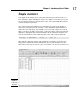
Chapter 1: Introducing Excel Tables Simple statistics Look again at the simple grocery list table that I mention earlier in the section, “What Is a Table and Why Do I Care?” See Figure 1-8 for this grocery list as I use this information to demonstrate some of the quick-and-dirty statistical tools that Excel provides. One of the slickest and quickest tools that Excel provides is the ability to effortlessly calculate the sum, average, count, minimum, and maximum of values in a selected range.
18 Part I: Where’s the Beef? The big question here, of course, is whether, with 9 different products but a total count of 14 items, you’ll be able to go through the express checkout line. But that information is irrelevant to our discussion. (You, however, might want to acquire another book I’m planning, Grocery Shopping For Dummies.) You aren’t limited, however, to simply calculating averages, counting entries, and summing values in your list. You can also calculate other statistical measures.
Chapter 1: Introducing Excel Tables simply adding, counting, or averaging the values in a table gives extremely useful insights. Sorting table records After you place information in an Excel table, you’ll find it very easy to sort the records. You can use the Sort A to Z button, the Sort Z to A button, or the Sort dialog box. Using the Sort buttons To sort table information by using a Sort buttons, click in the column you want to use for your sorting.
20 Part I: Where’s the Beef? 3. Select the first sort key. Use the Sort By drop-down list to select the field that you want to use for sorting. Next, choose what you want to use for sorting: values, cell colors, font colors, or icons. Probably, you’re going to sort by values, in which case, you’ll also need to indicate whether you want records arranged in ascending or descending order by selecting either the ascending A to Z or descending Z to A entry from the Order box.
Chapter 1: Introducing Excel Tables For a start, the Sort Options dialog box enables you to indicate whether case sensitivity (uppercase versus lowercase) should be considered. You can also use the Sort Options dialog box to tell Excel that it should sort rows instead of columns or columns instead of rows. You make this specification by using either Orientation radio button: Sort Top to Bottom or Sort Left to Right. Click OK when you’ve sorted out your sorting options. 6. Click OK.
22 Part I: Where’s the Beef? Drop-down list boxes appear when you turn on AutoFiltering. Figure 1-11: How an Excel table looks after using AutoFilter. To filter the list by using the contents of some field, select (or open) the drop-down list for that field. For example, in the case of the little workbook shown in Figure 1-11, you might choose to filter the grocery list so that it shows only those items that you’ll purchase at Sams Grocery. To do this, click the Store drop-down list down-arrow button.
Chapter 1: Introducing Excel Tables Figure 1-12: Sams and Sams alone. Undoing a filter To remove an AutoFilter, display the table menu by clicking a drop-down list’s button. Then choose the Clear Filter command from the table menu. Turning off filter The Data➪Filter command is actually a toggle switch. When filtering is turned on, Excel turns the header row of the table into a row of drop-down lists. When you turn off filtering, Excel removes the drop-down list functionality.
24 Part I: Where’s the Beef? Figure 1-13: The Custom AutoFilter dialog box. To create a custom AutoFilter, take the following steps: 1. Turn on the Excel Filters. As I mention earlier in this section, filtering is probably already on because you’ve created a table. However, if filtering isn’t turned on, select the table and then choose Data➪Filter. 2. Select the field that you want to use for your custom AutoFilter.
Chapter 1: Introducing Excel Tables The key thing to be aware of is that you want to pick a filtering operation that, in conjunction with your filtering criteria, enables you to identify the records that you want to appear in your filtered list. Note that Excel initially fills in the filtering option that matches the command you selected on the Text Filter submenu, but you can change this initial filtering selection to something else. In practice, you won’t want to use precise filtering criteria.
26 Part I: Where’s the Beef? If you want to filter the grocery list to show only the most expensive items that you purchase at Sams Grocery, for example, you might first filter the table to show items from Sams Grocery only. Then, working with this filtered table, you would further filter the table to show the most expensive items or only those items with the price exceeding some specified amount. The idea of filtering a filtered table seems, perhaps, esoteric.
Chapter 1: Introducing Excel Tables Figure 1-15: A table set up for advanced filters. To construct a Boolean expression, you use a comparison operator from Table 1-2 and then a value used in the comparison.
28 Part I: Where’s the Beef? In Figure 1-15, for example, the Boolean expression in cell A14 (>1), checks to see whether a value is greater than 1, and the Boolean expression in cell B14 (>=5) checks to see whether the value is greater than or equal to 5. Any record that meets both of these tests gets included by the filtering operation. Here’s an important point: Any record in the table that meets the criteria in any one of the criteria rows gets included in the filtered table.
Chapter 1: Introducing Excel Tables down arrow. This technique selects the Excel table range using the arrow keys. 2. Choose Data➪Advanced Filter. Excel displays the Advanced Filter dialog box, as shown in Figure 1-17. Figure 1-17: Set up an advanced filter here. 3. Tell Excel where to place the filtered table. Use either Action radio button to specify whether you want the table filtered in place or copied to some new location.
30 Part I: Where’s the Beef?