6-Series Multiparameter Water Quality Sondes User Manual 6-Series: 6600 V2 6600EDS V2 6920 V2 6820 V2 600 OMS V2 600XL 600XLM 600LS 600R 600QS
SAFETY NOTES TECHNICAL SUPPORT AND WARRANTY INFORMATION Contact information for technical support and warranty information on YSI’s Environmental Monitoring Systems products can be found in Section 9, Warranty and Service Information. COMPLIANCE When using the YSI 6-Series sondes in a European Community (CE) country, please be aware that electromagnetic compatibility (EMC) performance issues may occur under certain conditions, such as when the sonde is exposed to certain radio frequency fields.
TABLE OF CONTENTS SECTION 1 INTRODUCTION 1.1 ABOUT YSI 1.2 HOW TO USE THIS MANUAL 1.3 UNPACKING AND INSPECTION 1-1 1-1 1.2 SECTION 2 SONDES 2.1 GETTING STARTED 2.2 CONNECTING YOUR SONDE 2.3 PREPARING THE SONDE FOR USE 2.4 ECOWATCH FOR WINDOWS – GETTING STARTED 2.5 SONDE SOFTWARE SETUP 2.6 GETTING READY TO CALIBRATE 2.7 TAKING READINGS 2.8 USING ECOWATCH TO UPLOAD AND ANALYZE DATA 2.9 SONDE MENU 2.
5.14 CHLOROPHYLL 5.15 RHODAMINE 5.16 PHYCOCYANIN-CONTAINING BLUE-GREEN ALGAE 5.17 PHYCOERYTHRIN-CONTAINING BLUE-GREEN ALGAE 5.18 FLOW 5-21 5-28 5-31 5-37 5-42 SECTION 6 TROUBLESHOOTING 6.1 CALIBRATION ERRORS 6.2 SONDE COMMUNICATION PROBLEMS 6.3 SENSOR PERFORMANCE PROBLEMS 6-1 6-2 6-3 SECTION 7 COMMUNICATION 7.1 OVERVIEW 7.2 HARDWARE INTERFACE 7.3 RS-232 INTERFACE 7.4 SDI-12 INTERFACE 7-1 7-1 7-2 7.2 SECTION 8 UPGRADING SONDE FIRMWARE 8.1 SECTION 9 WARRANTY AND SERVICE INFORMATION 9.
Introduction Section 1 SECTION 1 INTRODUCTION 1.1 ABOUT YSI INCORPORATED From a three-man partnership in the basement of the Antioch College science building in 1948, YSI has grown into a commercial enterprise designing and manufacturing precision measurement sensors and control instruments for users around the world. Although our range of products is broad, we focus on three major markets: water testing and monitoring, health care, and bioprocessing.
Introduction Section 1 techniques, and system setup is necessary to obtain accurate and meaningful results. Thorough reading and understanding of this manual is essential to proper operation. Because of the many features, configurations and applications of these versatile products, some sections of this manual may not apply to the specific system you have purchased.
Sondes Section 2 SECTION 2 SONDES 2.1 GETTING STARTED The 6-Series Environmental Monitoring Systems from YSI are multi-parameter, water quality measurement, and data collection systems. They are intended for use in research, assessment, and regulatory compliance applications. Section 2 concentrates on sondes and how to operate them during different applications. A sonde is a torpedo-shaped water quality monitoring device that is placed in the water to gather water quality data.
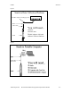
Sondes Section 2 2.2 CONNECTING YOUR SONDE There are a number of ways in which you may connect the sondes to various computers, data collection devices and VT-100 terminal emulators. To utilize the configuration that will work best for your application, make sure that you have all of the components that are necessary. The following list and diagrams (Figures 1-4) are a few possible configurations.
Sondes Section 2 Figure 2 Sonde to Data Collection Platform 6096 MS-8 Adapter with Flying Leads DCP MS-8 Field Cable You will need...
Sondes Section 2 Figure 4 Sonde to 650 Display/Logger YS Envir onmental Monitoring Systems 610-DM MS-8 650 MDS You will need... Field Cable + Sonde Field Cable - Sonde YS I 69 20 650 MDS Display/Logger YSI 650 operates on C-cells or rechargeable batteries.
Sondes Section 2 2.3 PREPARING THE SONDE FOR USE To prepare the sonde for calibration and operation, you need to install probes (sensors) into the connectors on the sonde bulkhead. In addition to probe installation, you need to install a new membrane on the YSI 6562 DO Probe if you are using this item. It is recommended that you install the DO membrane before installing the probe onto the bulkhead. For membrane changes in the future, you may be able to perform this operation without removing the DO probe.
Sondes Section 2 DO MEMBRANE INSTALLATION WITH THE PROBE NOT INSTALLED IN THE SONDE Remove the protective cap and the dry membrane from the YSI 6562 Dissolved Oxygen probe. Make sure that the protective cap is installed on the connector end of the probe. Do not allow the electrolyte solution to wet the probe‟s connector and O-ring seal areas. This solution is extremely corrosive to the connector and is difficult to remove.
Sondes Section 2 DO MEMBRANE INSTALLATION WITH THE PROBE INSTALLED IN THE SONDE Secure the sonde in a vertical position using a vise or a clamp and ring stand such that the sensors are upright. Remove the probe guard from the sonde. Remove the old DO membrane and clean the probe tip with water and lens cleaning tissue. Make sure to remove any debris or deposits from the O-ring groove.
Sondes Section 2 your fingers. Once the O-ring is in position, squeeze it every 90 degrees to equalize the tension. See Figure 11 above. DO NOT USE GREASE OR LUBICANT OF ANY KIND ON THE O-RING. Using a hobby knife or a scalpel, trim the excess Teflon from the membrane, making your cut about 1/8 inch below the O-ring as shown in Figure 12 below. A razor blade can be used for the cut if no knife or scalpel is available.
Sondes Section 2 REMOVING THE PORT PLUGS Using the long extended end of the probe installation tool supplied in the YSI 6570 Maintenance Kit, remove the port plugs. Save all the port plugs Figure 15 for possible future use. There are a variety of probe options for the sondes. Figures 15, 16 and 17 illustrate the uses of the common tool for port plug removal. Note that this tool will also be used to install the various probes.
Sondes Section 2 600XL & 600XLM SONDE BULKHEAD 3 Port Sonde: 1 Rapid Pulse DO, 1 Conductivity/Temperature, and 1 pH/ORP 6562 Dissolved oxygen probe = 3-pin connector 6560 Conductivity/Temperature = 6-pin connector 6561 pH probe = 4 pin connector 6565 Combo pH/ORP probe = 4 pin connector Figure 19 DISSOLVED OXYGEN 6562 CONDUCTIVITY/ TEMPERATURE 6560 ALL ISE PROBES 6600V2-2 SONDE BULKHEAD 8 Port Sonde: 1 Rapid Pulse DO, 1 Conductivity/Temperature, 2 Optical, 3 ISE, 1 pH/ORP Figure 20A
Sondes Section 2 6600EDS V2-2 SONDE BULKHEAD 5 Port Sonde: 1 Rapid Pulse DO, 1 Conductivity/Temperature, 2 Optical, 1 pH/ORP Figure 20B 6562 Dissolved oxygen probe = 3-pin connector 6560 Conductivity/Temperature = 6-pin connector 6561 or 6561FG pH probe = 4 pin connector 6565 or 6565FG pH/ORP probe = 4 pin connector 6566 Fouling Resistant pH/ORP probe = 4 pin connector 6026 Turbidity Probe, Wiping = 8 pin connector 6136 Turbidity Probe, Wiping = 8 pin connector 6025 Chlorophyll Pr
Sondes Section 2 6820V2-1 & 6920V2-1 SONDE BULKHEADS 7 Port Sonde: 1 Rapid Pulse DO, 1 Conductivity/Temperature, 1 Optical, 1 pH/ORP, 3 ISE 6562 Dissolved oxygen probe = 3-pin connector 6560 Conductivity/Temperature = 6-pin connector 6561 or 6561FG pH probe = 4 pin connector 6565 or 6565FG pH/ORP probe = 4 pin connector 6566 Fouling Resistant pH/ORP probe = 4 pin connector 6882 Chloride Probe = leaf spring connector 6883 Ammonium Probe = leaf spring connector 6884 Nitrate Pr
Sondes Section 2 600LS BULKHEAD If are working with a 600LS, all sensors will have been installed at the factory. Figure 21C Conductivity Depth Temperature 600R BULKHEAD If are working with a 600R sonde, your instrument will arrive with the probes installed. Figure 22 pH GLASS TEMPERATURE pH REFERENCE 6850 CONDUCTIVITY DISSOLVED OXYGEN 600QS BULKHEAD If are working with a 600QS sonde, your instrument will arrive with the probes installed.
Sondes Section 2 600 OMS V2-1 BULKHEAD The conductivity sensor (module/port) for the 600 OMS V2-1 is factory installed. Optical probes (turbidity, chlorophyll, rhodamine WT, ROX optical DO, BGA-PC, and BGA-PE) are threaded into the optical port on the bottom of the sonde by the user.
Sondes Section 2 INSTALLING THE TURBIDITY, CHLOROPHYLL, RHODAMINE WT , BGA-PHYCOCYANIN, BGAPHYCOERYTHRIN, AND ROX OPTICAL DISSOLVED OXYGEN PROBES If you are using any of optical probes listed, it is recommended that the optical sensors be installed first. If you are not installing one of these probes, do not remove the port plug, and go on to the next probe installation.
Sondes Section 2 INSTALLING THE ISE PROBES The Ammonium, Nitrate and Chloride ISE probes do not have slip nuts and should be installed without tools. Use only your fingers to tighten. Any ISE probe can be installed in any of the three ports labeled “3”, “4”, and “5” on the sonde bulkhead of the 6820V2-1, 6920V2-1, and 6600V2-2 sondes or the single ISE port on the 6820V2-2 and 6920V2-2 bulkheads.
Sondes 2.3.3 Section 2 STEP 3 - POWER Some type of external power supply is required to power the YSI 600R, 600QS, 600XL 6820V2-1, and the non-battery version of the 600 OMS V2-1sondes. The YSI 6920V2-1, 6920V2-2, 6600V2-2, 6600EDS V2-2, 6600V2-4, 600XLM, and battery version of the 600 OMS V2-1sondes have internal batteries or can run on external power.
Sondes Section 2 INSTALLING BATTERIES The 600XLM, 6600V2-2, 6600EDS V2-2, 6600V2-4, 6920V2-1, 6920V2-2 and battery version of the 600 OMS V2-1are the sondes that use alkaline batteries for power. A set of batteries is supplied with each of these sondes. If you do not have one of these sonde model types, you may skip this section. INSTALLING BATTERIES INTO THE YSI 600XLM OR 600 OMS V2-1 SONDES To install 4 AA-size alkaline batteries into the sonde, refer to the following directions and Figure 33.
Sondes Section 2 INSTALLING BATTERIES INTO THE YSI 6600V2-2, 6600EDS V2-2, AND 6600V2-4 SONDES IMPORTANT SAFETY FEATURE: The 116003 battery lid for the 6600V2-2, 6600EDS V2-2, and 6600V2-4 is equipped with a safety pressure-release valve. The valve will vent off any pressure build up in the battery compartment from waste gas that could be created by battery failure, improperly marked or installed batteries, flooding, and dead or heavily discharged batteries.
Sondes 2. Section 2 Press two of the outermost retaining tabs down into the groove. It should be clear that the retaining tabs have recessed into the groove along with the seal so that the tabs outermost edges are at or below the battery lid‟s mounting surface. Press tabs into groove Figures 35C and 35D 3. Press the remaining two outermost retaining tabs into the groove and check to make sure the tabs have been recessed as before.
Sondes Section 2 cannot be reset and the battery lid must be replaced before sonde deployment. Contact YSI Technical Support for instructions. Figure 35M: Closed valve OK to Deploy Figure 35N: Open valve DO NOT Deploy Lightly lubricate the o-rings on the outside of the battery cover. DO NOT lubricate the orange internal oring. Return the battery lid and HAND tighten the screws with the hex driver until snug. DO NOT OVER TIGHTEN.
Sondes Section 2 Check the O-rings and sealing surfaces for any contaminants that could interfere with the seal of the battery chamber. CAUTION: Make sure that there are NO contaminants between the O-ring and the sonde. Contaminants that are present under the O-ring may cause the O-ring to leak when the sonde is deployed. BATTERY CAP BULKHEAD CONNECTOR BAIL - + + - Lightly lubricate the o-rings on the bottom of the threads and on the connector stem as shown in Figure 37.
Sondes Section 2 CAUTION: The 6067B cable is for laboratory use only -- it is not waterproof and should not be submersed! Sondes that are equipped with level sensors use vented cables. See Appendix G, Using Vented Level, for detailed information.
Sondes Section 2 2.4 ECOWATCH FOR WINDOWS -GETTING STARTED This section will describe how to get started with EcoWatch for Windows, but detailed information is provided in Section 4, EcoWatch for Windows, or a convenient Windows Help section that is part of the software. It is recommended that you thoroughly read Section 4 or use the Help function for a comprehensive understanding of EcoWatch for Windows. 2.4.
Sondes Section 2 2.5 SONDE SOFTWARE SETUP There are two sets of software at work in any YSI environmental monitoring system. One is resident in your PC and is called EcoWatch for Windows. The other software is resident in the sonde itself. In this section, you will first make sure that the language associated with your sonde software is appropriate to your application and change it if necessary.
Sondes Section 2 Set the Comm port number to match the port to which you connected the sonde cable and make sure that the “This is an ADV6600” selection is NOT checked. NEXT, SELECT THE LANGUAGE (ENGLISH, FRENCH, OR GERMAN) WHICH WILL BE USED IN YOUR SONDE MENUS. Then click on the Start Code Update button. An indicator bar will show the progress of the upgrade as shown below.
Sondes Section 2 Figure 39 If your sonde has previously been used, the Main menu (rather than the # sign) may appear when communication is established. In this case simply proceed as described below. You will not be required to type “Menu”. If you are unable to establish interaction with the sonde, make sure that the cable is properly connected. If you are using external power, make certain that the YSI 6651 or 6038 power supply or other 12 vdc source is properly working.
Sondes Section 2 Figure 40 - Sonde Menu Flow Chart SONDE MENU FLOW CHART Sonde 1. Run 1. Conductivity 1. Discrete sample 2. DO % 2. Unattended sample 3. DO mg/L 2. Calibrate 4. Others 1. Directory 3. File 4. Status 5. System Date and Time 2. Upload Battery Voltage 3. Quick Upload Available Memory 1. Date & Time Logging Status 2. Comm Setup 4. View File 5. Quick View File 3. Page Length 1. () Date 4. Instrument ID 2. () Time 5. SDI-12 Address 3. () Temp, C 6.
Sondes Section 2 Select 1-Date & time. An asterisk will appear next to each selection to confirm the entry. Press 4 and 5 to activate the date and time functions. Pay particular attention to the date format that you have chosen when entering date. You must use the 24-hour clock format for entering time. Option 4- ( ) 4 digit year may be used so that the date will appear with either a two or four digit year display.
Sondes Section 2 ENABLING SENSORS To activate the sensors that are in your sonde, select Sensor from the Sonde Main menu. ------------Sensors enabled-----------1-(*)Time 2-(*)Temperature 3-(*)Conductivity 4-(*)Dissolved Oxy 5-(*)ISE1 pH 6-(*)ISE2 Orp 7-(*)ISE3 NH4+ 8-(*)ISE4 NO39-( )ISE5 NONE A-(*)Optic T Turbidity - 6136 B-(*)Optic C Chlorophyll Select option (0 for previous menu): Note that the exact appearance of this menu will vary depending upon the sensors that are available on your sonde.
Sondes Section 2 --------------Report setup------------1-(*)Date m/d/y E-(*)Orp mV 2-(*)Time hh:mm:ss F-(*)NH4+ N mg/L 3-(*)Temp C G-( )NH4+ N mV 4-(*)SpCond mS/cm H-( )NH3 N mg/L 5-( )Cond I-(*)NO3- N mg/L 6-( )Resist J-( )NO3- N mV 7-( )TDS K-(*)Cl- mg/L 8-( )Sal ppt L-( )Cl- mV 9-(*)DOsat % M-(*)Turbid+ NTU A-(*)DO mg/L N-(*)Chl ug/L B-( )DOchrg O-(*)Chl RFU C-(*)pH P-(*)Battery volts D-( )pH mV Select option (0 for previous menu): Note that the exact appearance of this menu will vary depending upon th
Sondes Section 2 CHECKING ADVANCED SETTINGS Select Advanced from the Main menu. The following menu will be displayed. ----------------Advanced-------------1-Cal constants 2-Setup 3-Sensor 4-Data filter Select option (0 for previous menu): Select Setup from the Advanced menu.
Sondes Section 2 ------------Advanced sensor----------1-TDS constant=0.65 2-Latitude=40 3-Altitude Ft=0 4-(*)Fixed probe 5-( )Moving probe 6-DO temp co %/C=1.1 7-DO warm up sec=40 8-( )Wait for DO 9-Wipes=1 A-Wipe int=5 B-SDI12-M/wipe=1 C-Turb temp co %/C=0.
Sondes Section 2 2.6 GETTING READY TO CALIBRATE 2.6.1 INTRODUCTION HEALTH AND SAFETY Reagents that are used to calibrate and check this instrument may be hazardous to your health. Take a moment to review health and safety information in Appendix A of this manual. Some calibration standard solutions may require special handling.
Sondes Section 2 6. Have several clean, absorbent paper towels or cotton cloths available to dry the sonde between rinses and calibration solutions. Shake the excess rinse water off of the sonde, especially when the probe guard is installed. Dry off the outside of the sonde and probe guard. Making sure that the sonde is dry reduces carry-over contamination of calibrator solutions and increases the accuracy of the calibration. 7.
Sondes Section 2 RECOMMENDED VOLUMES OF CALIBRATION REAGENTS The approximate volumes of the reagents are specified below for both the upright and inverted orientations. Note that the volume values are only estimates. The actual amount of calibrator solution required will depend on how many and what type of other probes are installed in you sonde bulkhead.
Sondes Section 2 Table 6 6600V2-4 Sonde with Standard Long Calibration Cup**** Probe to Calibrate Upright Conductivity 525ml pH/ORP 500ml All Optical Sensors 425ml Inverted 150ml 150ml DO NOT CALIBRATE*** Table 7 600 OMS V2-1 Sonde* * Probe to Calibrate Upright Conductivity 375ml Turbidity, Chlorophyll, Rhodamine WT 350ml Inverted N/A N/A Table 8 600R and 600QS Sondes Probe to Calibrate Upright Inverted Conductivity 350ml N/A pH/ORP 120ml N/A * See section below for special instructions dealing with c
Sondes Section 2 NOTE CAREFULLY: All optical sensors MUST be calibrated in the upright position no matter which type of calibration cup is employed. In the upside-down position, the meniscus of the standard causes a great deal of interference and this interference is likely to result in calibration errors and/or erroneous field readings.
Sondes Section 2 3. Note that the exact appearance of this menu will vary depending upon the sensors that are available and enabled on your sonde. To select any of the parameters from the Calibrate menu, input the number that is next to the parameter. Once you have chosen a parameter, some of the parameters will have a number that appears in parentheses. These are the default values and will be used during calibration if you press Enter without inputting another value.
Sondes Section 2 Note that all parameters that have been enabled will appear - not just the one being calibrated at the moment. The user should carefully observe the stabilization of the readings of the parameter that is being calibrated and, when the readings are stable for approximately 30 seconds, press Enter to implement the calibration and the following message will appear. Calibrated. Press to continue. NOTE: If an ERROR message appears, begin the calibration procedure again.
Sondes Section 2 NOTE: The YSI conductivity system is very linear over its entire 0-100 mS/cm range. Therefore, it is usually not necessary to use calibration solutions other than the 10 mS/cm reagent recommended above for all environmental applications from low conductivity freshwater to seawater. YSI does offer the 3161 (1 mS/cm) and 3165 (100 mS/cm) conductivity standards for users who want to assure maximum accuracy at the high and low ends of the sensor range.
Sondes Section 2 Monitoring Applications If your instrument will be used in monitoring applications where data is being captured at a longer interval (e.g. 15 – 60 minutes) to internal sonde memory, a data collection platform or a computer, you need to activate “Autosleep RS232” as described in Section 2.5, Sonde Software Setup. Then follow the instructions detailed above for the Sampling Application calibration.
Sondes Section 2 DEPTH AND LEVEL For the depth and level calibration, make certain that the depth sensor module is in air and not immersed in any solution. From the Calibrate menu, select Pressure-Abs (or Pressure-Gage if you have a vented level sensor) to access the depth calibration procedure. Input 0.00 or some known sensor offset in feet. Press Enter and monitor the stabilization of the depth readings with time.
Sondes Section 2 The next calibration instructions are only for the ISE sensors which are options for the 6820V2-1, 6800V2-2, 6600V2-2, 6920V2-1, and 6920V2-2 sondes. If you do not have one of these sondes, you may skip to the next section. AMMONIUM (NH4+) , CHLORIDE CL- AND NITRATE (NO3-) 3-POINT WARNING: AMMONIUM AND NITRATE SENSORS CAN ONLY BE USED AT DEPTHS OF LESS THAN 50 FEET (15 METERS). USE OF THE SENSORS AT GREATER DEPTHS IS LIKELY TO PERMANENTLY DAMAGE THE SENSOR MEMBRANE.
Sondes Section 2 CALIBRATION TIP: Exposure to the high ionic content of pH buffers can cause a significant, but temporary, drift in these ISE probes (ammonium, nitrate and chloride probes). Therefore, when calibrating the pH probe, YSI recommends that you use one of the following methods to minimize errors in the subsequent readings: Calibrate pH first, immersing all of the probes in the pH buffers.
Sondes Section 2 water. Input the value 0 NTU at the prompt, and press Enter. The screen will display real-time readings that will allow you to determine when the readings have stabilized. Activate the wiper 1-2 times by pressing 3-Clean Optics as shown on the screen, to remove any bubbles. After stabilization is complete, press Enter to “confirm” the first calibration and then, as instructed, press Enter to continue.
Sondes Section 2 Before making any field readings, carefully read Section 5.16, Principles of Operation to better understand the practical aspects of BGA-PC fluorescence measurements. To begin the calibration, place the correct amount (see Tables 1-8 above) of clear deionized or distilled water into the YSI clear calibration cup provided. Immerse the sonde in the water. Input the value 0 cells/mL at the prompt, and press Enter.
Sondes Section 2 RHODAMINE WT 2-POINT Select Rhodamine from the Calibrate Menu and then 2-2-Point. NOTE: One standard must be 0 ug/L in rhodamine WT, and this standard must be calibrated first. To begin the calibration, place the correct amount (see Tables 1-8) of 0 standard (clear deionized or distilled water) into the calibration cup provided with your sonde and immerse the sonde in the water. Input the value 0 ug/L at the prompt, and press Enter.
Sondes Section 2 2.7 TAKING READINGS After you have (1) enabled the sensors, (2) set the report to show the parameters that you want to see, and (3) calibrated the sensors, you are now ready to take readings. There are two basic approaches to sampling, discrete and unattended. Using discrete sampling, the sonde is connected via a communication cable to a PC or 650 MDS Display/Logger.
Sondes Section 2 If you started sampling without entering a filename, the default name NONAME1 will be assigned to your file. Whenever you press 1-LOG last sample or 2-LOG ON/OFF from the menu, NONAME1 will be opened during sampling. If this happens, and you want to restart the file with a different name, press 5-Close file and rename the file. Select 4-Site to assign a site name with a maximum of 31 characters. This allows you to enter the name of the site where you are sampling.
Sondes Section 2 sampling at 6:00 PM on July 31, 1996. The site is Clear Lake, near the spillway, and you want to log all of the readings to a single file CLRLAKE3. ------------Unattended setup----------1-Interval=00:15:00 2-Start date=07/17/96 3-Start time=18:00:00 4-Duration days=365 5-File= 6-Site= 7-Bat volts: 11.6 8-Bat life 25.1 days 9-Free mem 41.3 days A-1st sample in 8.
Sondes Section 2 Skip B-View params to log in this initial test study. This feature will be explained in detail in Section 2.9, Sonde Menu. After making the above entries, the sonde software will automatically calculate the expected battery life, and the time it will take for the sonde memory to be filled. This information is displayed on the screen for your consideration as items 8, 9, and A.
Sondes Section 2 ----------------Logging---------------1-Interval=00:15:00 2-Next at 07/17/96 3-Next at 18:00:00 4-Stop at 07/31/96 5-Stop at 18:00:00 6-File=clrlake3 7-Site=Clear Lake at Spillway 8-Bat volts: 11.7 9-Bat life 25.5 days A-Free mem 41.3 days B-Stop logging C-Show Live Data Select option (0 for previous menu): The display now shows the next date and time for logging, and the stop date and time for the logging study.
Sondes Section 2 2.8 USING ECOWATCH TO CAPTURE, UPLOAD AND ANALYZE DATA EcoWatch for Windows software is reporting and plotting software for use with the YSI 6-Series sondes. Instructions for installing this software were included in Section 2.1, Getting Started. This program can also be used to upload and view data logged to sonde memory during either discrete or unattended sampling. CAPTURE EcoWatch for Windows can be used to capture data in real-time to your PC‟s hard drive or to a floppy disk.
Sondes Section 2 -----------------File----------------1-Directory 4-View file 2-Upload 5-Quick view file 3-Quick Upload 6-Delete all files Select option (0 for previous menu): 1 Select 1-Directory to view all files currently stored in the sondes flash disk memory, the screen below shows 6 files. All data files (.dat extension) could be uploaded to EcoWatch for viewing or plotting, but you do not need to upload all files in the directory. The file with the .
Sondes Section 2 --------------Time window-------------1-Proceed 2-Start date=08/14/96 3-Start time=18:00:00 4-Stop date=08/28/96 5-Stop time=11:00:00 Select option (0 for previous menu): Select 1-Proceed. Choose the appropriate file transfer protocol (in this example, PC6000) and a status box will show the progress of the upload.
Sondes Section 2 Select 5-Quick view file to view the last page of data from the last data file in flash disk memory. This feature is particularly useful to quickly review any recently acquired data so that system performance can be assessed. Select 6-Delete all files to IRREVERSIBLY remove all files (INCLUDING the .glp file that contains calibration information) from the sonde flash disk memory.
Sondes Section 2 Figure 41 Opening a File Some daily variations may be noticed in parameters such as dissolved oxygen, pH and temperature in this particular study. This is fairly typical in many natural bodies of water. Note also that conductivity is low at both ends of the graph. You may notice similar perturbations in some of the other readings as well. In this example, the sonde was not in the water for a short time at the beginning and end of the study.
Sondes Section 2 Figure 42 Viewing Options It may be somewhat awkward to scan the data table in this manner; therefore you have the option to turn off the graphical representation and allow the table to fill the window. See Figure 43. Notice now that when you click on View, the Graph item is no longer checked.
Sondes Section 2 Figure 43 Viewing the Data in Table Format Viewing features such as Grid, Marker, Zoom In, Zoom Out and Unzoom are all available when you activate the Graph function. Give each a try as you practice and learn more about the many features of EcoWatch. The Statistics and Study functions of EcoWatch are shown in Figure 44. Both provide overview information related to the study data.
Sondes Section 2 Figure 44 Statistics and Study Information Next, with the Statistics and Study windows closed, return to the View menu, close Table and activate Graph. Using the right mouse button, click at any point on the graph. A dotted vertical line appears along with specific data values in boxes to the left of the displayed graphs, as shown in Figure 45. You can hold down the right mouse button and move the mouse to scan the entire graph that is displayed in the window.
Sondes Section 2 Figure 45 Viewing the Data with Right-Button Mouse Function CHANGING DISPLAY FORMATS USING SETUP Beyond selecting data viewing options such as table format or graphical format, you may also customize your data displays. For example, you may change the order in which parameters are viewed, you may add and delete parameters, you may change plot appearance using different interval times and different units, and you may change the x-axis if you prefer a parameter other than date or time.
Sondes Section 2 Figure 46 Changing the Appearance of a Graph or Table If you are displaying the graph, you may change the appearance by changing font, font style, size and text color. You may also change page color, trace color and graph background color. You may assign a custom 2-line title for the graph, and finally, you may display 1 trace or 2 per set of axes. For display of table formatted results you may change font, font style, size and text color.
Sondes Section 2 along the x-axis, you may also manually scale the y-axis. This may allow you to discard a noise spike and obtain better resolution of events unrelated to the noise. Functions like Autoscale, Redraw and Cancel Limits are all used to “undo” some of the customization functions. Below in Figure 47 you see some of these functions. One very commonly used function is Limit Data Set.
Sondes Section 2 Figure 48 Using Limit Data Set to Display a Subset of Data To return to the full set of data again, click on Graph, then Cancel Limits. If you desire a hard copy of any graph or table, or even a subset expression as shown above, you may use the Edit, Copy command to „copy‟ the graph in the active window to the “Clipboard”. You can then „paste‟ this graph to the Windows application program of your choice. You may also be able to print graphs and tables as described in the next section.
Sondes Section 2 Figure 49 Saving, Exporting, Printing and Related Functions EXAMPLE OF CUSTOMIZING A SUBSET OF SAMPLE.DAT To conclude this section we have used a few of the many tools available in EcoWatch to demonstrate how you might use this powerful plotting and reporting program to express study results. We encourage you to try some of the tools and learn more about EcoWatch by using the Window‟s Help function, which is available when the EcoWatch program is running. Using SAMPLE.
Sondes Section 2 Figure 50 Customizing a Graph from SAMPLE.DAT Finally, we selected File|Save Data Display and gave the custom plot the name “4PARAM” to that the presentation can be immediately recalled in the future. As you become more familiar with EcoWatch for Windows, the plotting, analysis and reporting functions can be accomplished easily and quickly. Practice with all of the functions and, again, do not forget to use Window‟s Help for more detail, or see Section 4, EcoWatch for Windows.
Sondes Section 2 2.9 SONDE MENU The functions of the sondes are accessible through the sonde menu. The sonde menu structure makes it simple and convenient to select functions. This section provides a description of the menus and their capabilities. When moving between menus within the sonde software structure, use the 0 or Esc to back up to the previous menu. To exit menus and return to the sonde command line (the # sign), press 0 or Esc until the question “Exit menu (Y/N)?” appears.
Sondes Section 2 2.9.1 RUN Select 1-Run from the Main menu to begin taking readings or to set/verify the parameters required for a study. There are two options in the Run menu. ---------------Run setup--------------1-Discrete sample 2-Unattended sample Select option (0 for previous menu): 1 DISCRETE SAMPLING Discrete sampling is usually used in short term, spot sampling applications when the user is present at the site and the unit is attached to a 650 MDS Display/Logger or laptop PC.
Sondes Section 2 Select 1 – Start sampling option to start discrete sampling. After the initial sampling time interval has passed (4 seconds in the screen above), sequential lines of data will appear on the screen.
Sondes Section 2 Sampling Faster Than 0.5 Seconds For special applications, your sonde is capable of faster sampling. The only limitation is a reduction of the number of sensors selected. To determine the maximum sampling frequency for your sensor setup, divide 36 by the number of enabled sensors in addition to the DO sensor. Example: If you enable any three sensors plus DO, divide 36 by 3 to obtain 12 samples/second (12 Hz) or 0.083 seconds between samples as the maximum sampling frequency.
Sondes Section 2 ------------Unattended setup----------1-Interval=00:15:00 2-Start date=07/17/96 3-Start time=18:00:00 4-Duration days=14 5-File=clrlake3 6-Site=Clear Lake at Spillway 7-Bat volts: 9.1 8-Bat life 21.2 days 9-Free mem 18.9 days A-1st sample in 8.
Sondes Section 2 Select B-View Parameters to log to confirm that your sensor and report setups are configured correctly as described in Sections 2.9.6 and 2.9.7. An example screen is shown below.
Sondes Section 2 Select 1-Yes and the screen will change. ----------------Logging---------------1-Interval=00:15:00 2-Next at 07/17/96 3-Next at 18:00:00 4-Stop at 07/31/96 5-Stop at 18:00:00 6-File=clrlake3 7-Site=Clear Lake at Spillway 8-Bat volts: 9.0 9-Bat life 21.2 days A-Free mem 18.9 days B-Stop logging C-Show Live Data Select option (0 for previous menu): The display now shows the next date and time for logging and the stop date and time for the logging study.
Sondes Section 2 2.9.2 CALIBRATE All of the sonde sensors (except temperature) require periodic calibration to assure high performance. However, the calibration protocols for Rapid Pulse Polarographic dissolved oxygen are significantly different depending on whether the sonde is being set up for spot sampling or longer term unattended monitoring studies.
Sondes Section 2 ---------------Calibrate-------------1-Conductivity 6-ISE3 NH4+ 2-Dissolved Oxy 7-ISE4 NO33-Pressure-Abs 8-ISE5 Cl4-ISE1 pH 9-Optic T-Turbidity 6136 5-ISE2 ORP A-Optic C - Chlorophyll Select option (0 for previous menu): CONDUCTIVITY Select 1-Conductivity to calibrate the conductivity probe and a second menu will offer you the options of calibrating in specific conductance, conductivity, or salinity. Calibrating any one option automatically calibrates the other two.
Sondes Section 2 For the mg/L mode, calibration is carried out in a water sample which has a known concentration of dissolved oxygen, usually determined by Winkler titration. For this calibration procedure, the sensor should be immersed in the water. After thermal equilibration, enter the known mg/L value, press Enter, and the calibration procedure will be carried out automatically as for the percent saturation mode above.
Sondes Section 2 membrane installed on the 6150 probe and NOT a function of the probe, i.e., the constants reflect the characteristics of the sensor membrane and NOT the probe. When a 6150 probe is purchased from YSI, it already has a sensor membrane installed and the constants of that membrane are transferred automatically to the sonde PCB when the sensor is run for the first time.
Sondes Section 2 which characterize the new membrane and they MUST be entered via the Calibrate|Optic X – Dissolved Oxy|Enter Cal Sheet selection as show above. Once the new constants have been entered in coded form they will be transferred to the probe and will be visible in uncoded form in Advanced|Cal Constants. See Section 5.9, Principles of Operation and Appendix M, ROX Optical DO Sensor for more information.
Sondes Section 2 Calibration Using mg/L – 1-Point Place the sensor in a container which contains oxygen of a known concentration of dissolved oxygen in mg/L AND THAT IS WITHIN +/- 10% of AIR SATURATION as determined by one of the following methods: Winkler titration Aerating the solution and assuming that it is saturated, or Measurement with another instrument.
Sondes Section 2 NOTE CAREFULLY: If you used sodium sulfite solution as your zero calibration medium, you MUST carefully remove all traces of the reagent from the probes prior to proceeding to the second point. YSI recommends that the second calibration point be in air-saturated water if you use sodium sulfite solution as your zero oxygen medium.
Sondes Section 2 pH When selecting ISE1 pH, you will be given the choice of 1-point, 2-point, or 3-point calibrations. Select the 1-point option only if you are adjusting a previous calibration. If a 2-point or 3-point calibration has been performed previously, you can adjust the calibration by carrying out a one point calibration. Immerse the sonde in a buffer of known pH value and press Enter. You will be prompted to type in the pH value of the solution.
Sondes Section 2 When selecting ISE3-NH4+, you will be given the choice of 1-point, 2-point, or 3-point calibrations for your ammonium (NH4+) sensor. Select the 1-point option only if you are adjusting a previous calibration. If a 2-point or 3-point calibration has been performed previously, you can adjust the calibration by doing a one point calibration. Immerse the sonde in any solution of known ammonium concentration and press Enter.
Sondes Section 2 CHLORIDE When selecting ISE5-CL-, you will be given the choice of 1-point, 2-point, or 3-point calibrations for your chloride (Cl-) sensor. The procedure is identical to that for the ammonium sensor, except that the calibrant values are in mg/L of Cl instead of NH4-N. IMPORTANT: We recommend that the user employ standards for chloride that are 10 times greater than for ammonium and nitrate.
Sondes Section 2 When selecting Optic X -6026-Turbidity (or 6136-Turbidity), there will be a choice of 1-point, 2-point, or 3-point calibrations for your turbidity sensor. The 1-point option is normally used to zero the turbidity probe in 0 NTU standard. Place the sonde in clear water (deionized or distilled) with no suspended solids, and input 0 NTU at the screen prompt.
Sondes Section 2 Enter after the readings have stabilized to confirm the calibration and zero the sensor. Then, press any key to return to the Calibrate menu. If you select Chl µg/L in the initial calibration routine, there will be a choice of 1-point, 2-point, or 3-point options. The 1-point selection is normally used to zero the fluorescence probe in a medium that is chlorophyll-free.
Sondes Section 2 To calibrate your 6131 Blue-Green Algae-Phycocyanin (BGA-PC) sensor, select BGA-PC cells/mL in the initial calibration routine. There will be a choice of 1-point or 2-point options. The 1-point selection is normally used to zero the fluorescence probe in a medium that is BGA-free. If you use this method, you will either choose to utilize the default sensitivity for BGA-PC in the sonde software or to update a previous 2-point calibration.
Sondes Section 2 determining the BGA-PC content of algal suspensions by using standard cell counting techniques. See Section 5.17, Principles of Operation of this manual for more information about BGA-PC standards. Select the 2-point option to calibrate the BGA-PE probe using two calibration standards. In this case, one of the standards must be clear water (0 cells/mL) and the other should be in the range of the suspected BGA-PC content at the environmental site.
Sondes Section 2 point calibration, but the software will prompt you to place the sonde in the additional solution to complete the 3-point procedure. For all rhodamine calibration procedures, be certain that the standard and sensor are thermally equilibrated prior to proceeding with the calibration.
Sondes Section 2 CALIBRATION RECORD – THE GLP FILE When any sensor is calibrated, 6-series sondes will automatically create a file in sonde memory that provides details of the calibration coefficients before and after the calibration. The file will have a .glp extension and will have the Circuit Board Serial # as the default filename. The file can be viewed by following the path File|Directory|View from the Main sonde menu. -------------File details-------------1-View file 2-File:00003001.
Sondes Section 2 Pressing 1-View file will show the calibration record for the sonde.
Sondes Section 2 Constants and is described in Section 2.9.8. All other values in the .glp file are equivalent to those shown in the Advanced|Cal Constants menu. CAUTION: Calibration records for all sensors will automatically be stored in the .glp file until the Delete All Files command is used from the File menu. However, if the Delete command is issued, all files, including the .glp (calibration record) file will be lost. Therefore, it is extremely important to remember to upload the .
Sondes Section 2 PC6000 format will transfer the data so that it will be compatible with the EcoWatch for Windows (supplied with your sonde) software package. YSI recommends data transfer in this format since it is significantly more rapid than other transfer options. If this data is required in Comma & Quote Delimited and/or ASCII formats, the user can quickly generate data in these formats using the Export function in EcoWatch for Windows.
Sondes Section 2 You may choose the entire file. Use the Space Bar to alternately stop and to resume scrolling. Use the Esc key to cancel the view. Select the 5–Quick View File option to view the last page of data from the last data file in sonde memory. This feature is particularly useful in quickly reviewing recently acquired data at field sites so that system performance can be assessed. Select 6–Delete all files to IRREVERSIBLY remove all files from the sonde memory (INCLUDING the .
Sondes Section 2 2.9.4 STATUS Select 4-Status from the Sonde Main menu to obtain general information about the sonde and its setup. -----------------Status---------------1-Version:3.01 2-Date=07/22/96 3-Time=09:04:28 4-Bat volts: 9.0 5-Bat life 21.2 days 6-Free bytes:129792 7-Logging:Inactive Select option (0 for previous menu): 1-Version identifies the specific version of sonde software loaded in the sonde. This number is especially useful if you are calling YSI Technical Support.
Sondes Section 2 2.9.5 SYSTEM Select 5-System from the Sonde Main menu to set the date and time, customize the sonde communication protocol, adjust how information appears on the screen, and enter an instrument identification number and a GLP file designation. 1-Date & time 2-Comm setup 3-Page length=25 4-Instrument ID=YSI Sonde 5-Circuit board SN:00003001 6-GLP filename=00003001 7-SDI-12 address=0 Select option (0 for previous menu): Select Date & time.
Sondes Section 2 The default is 9600, but you may change it to match your host communication interface protocol by typing in the corresponding number, 1 through 7. An asterisk confirms the selection. Auto baud may be selected along with any of the choices. The Auto baud option allows the sonde to recognize and adjust to the received characters and we recommend that it is activated.
Sondes Section 2 -------------Report 1-(*)Date 2-(*)Time hh:mm:ss 3-(*)Temp C 4-(*)SpCond uS/cm 5-( )Cond 6-( )Resist 7-( )TDS 8-( )Sal ppt 9-(*)DOsat % A-(*)DOsat %Local B-( )DO mg/L setup-------------C-( )DOchrg D-( )pH E-( )pH mV F-(*)Orp mV G-( )PAR1 H-( )PAR2 I-(*)Turbid+ NTU J-(*)Chl ug/L K-( )Chl RFU L-(*)Battery volts Select option (0 for previous menu): The asterisks (*) that follow the numbers or letters indicate that the parameter will appear on all outputs and reports.
Sondes Section 2 Oxygen in % air saturation, Dissolved Oxygen in mg/L, pH, ORP in millivolts, Turbidity in NTUs and Chlorophyll in ug/L. Date and time will also be displayed. NOTE: Do not attempt to memorize or associate a number or letter with a particular parameter. The numbering scheme is dynamic and changes depending on the sensors which have been enabled. The following list is a complete listing of the abbreviations utilized for the various parameters and units available in the Report setup menu.
Sondes PAR1 PAR 2 Section 2 Output from special photosynthetically active radiation sensor in mv or Photon Flux Density in umoles/sec/m2 Output from special photosynthetically active radiation sensor in mv or Photon Flux Density in umoles/sec/m2 2.9.7 SENSOR The Sensor menu allows you to Enable or Disable (turn on or off) any available sensor and, in some cases, to select the port in which your sensor is installed. From the Sonde Main menu select 7-Sensor and the following display will appear.
Sondes Section 2 As noted above, the ISE3 PAR1 selection is used in a special instrument mated to a sensor for Photosynthetically Active Radiation that is available from Endeco/YSI. See Section 9 for contact information and Appendix K for a brief description of the PAR system for potential users. A submenu similar to that below will appear if any of the Optic options (T, C, B, or O) is chosen as a port for a particular optical sensor..
Sondes Section 2 Select 1-Cal constants to display the calibration constants, as shown in the following example. Note that values only appear for the enabled sensors. -------------Cal constants------------1-Cond:5 B-NO3 A:2.543 2-DO gain:1.3048 C-Cl J:99.5 3-mV offset:0 D-Cl S:-0.195 4-pH offset:0 E-Cl A:2.543 5-pH gain:-5.05833 F-Turb Offset:0 6-NH4 J:51.2 G-Turb A1:500 7-NH4 S:0.195 H-Turb M1:500 8-NH4 A:1.092 I-Turb A2:1000 9-NO3 J:99.5 J-Turb M2:1000 A-NO3 S:-0.
Sondes Turb+ A2 Turb+ M2 Chl Offset Chl A1 Chl M1 Chl A2 Chl M2 Chl RFU Offset PC Offset PC Gain PC RFU Offset PE Offset PE Gain PE RFU Offset Rhod Offset Rhod A1 Rhod M1 Rhod A2 Rhod M2 Section 2 1000 0.6 to 1.5 Range is ratio of (M2-M1) to (A2-A1) 0 500 500 1000 1000 0 0 1 0 0 1 0 0 500 500 1000 1000 -30 to 20 0.6 to 1.5 Range is ratio of M1 to A1 0.6 to 1.5 Range is ratio of (M2-M1) to (A2-A1) -0.1 to +0.1 -5000 to 10000 Not checked Not checked -5000 to 15000 Not checked Not checked -10 to 10 0.
Sondes Section 2 ------Start up:--------------1-(*)Normal 2-( )Menu 3-( )Run 4-( )Menu Run 5-( )NMEA Select option (0 for previous menu): Users should select the option for their application based on the descriptions below. Note, however, that the “Start up Normal” selection will be best for most applications. 1- ( ) Start up Normal. This selection is the factory default and should be used for most operations of the sonde.
Sondes Section 2 6-( ) Multi SDI12. Modifies the SDI12 protocol as follows: (1) No SDI12 service request will be issued. (2) Break commands will not cause a measurement reading to be aborted. Normally, you should leave this feature “off”. 7-( ) Full SDI12. Enabling this feature forces full SDI-12 specification in order to pass the NR Systems SDI-12 Verifier. Disabling this feature will allow the unit to be more fault tolerant and will save some power. We recommend that you leave this feature “off”.
Sondes Section 2 ------------Advanced sensor----------1-TDS constant=0.65 2-Latitude=40 3-Altitude Ft=0 4-(*)Fixed probe 5-( )Moving probe 6-DO temp co %/C=1.1 7-DO warm up sec=40 8-(*)Wait for DO 9-Wipes=1 A-Wipe int=1 B-SDI12-M/wipe=1 C-Turb temp co %/C=0.3 D-(*)Turb spike filter E-Chl temp co %/C=0 Select option (0 for previous menu): NOTE: The number of items on this menu depends greatly on the sensors that are available and enabled on your sonde. Below we describe every possible item on this menu.
Sondes Section 2 calculation of depth or level. This item will only appear if the pressure sensor is enabled in the Sensors menu. (*)Fixed probe This selection allows you to identify how your sonde is being used. If your sonde is “fixed” or secured to a dock, buoy, platform or similar, select this option. This information is used in the calculation of depth and level. This item will only appear if the Pressure-Abs sensor is enabled in the Sensors menu.
Sondes Section 2 activated at the interval assigned in the Unattended setup rather than that assigned in Wipe Int. Thus, in an Unattended study setup at a 15 minute sampling interval, the wiper will be activated only once every 15 minutes rather than at the indicated Wipe Int of 1 minute. CAUTION: If Wipe Int is set to zero, then no wiping will occur either in Discrete or Unattended Sampling.
Sondes Section 2 Sondes with no optical (turbidity, chlorophyll, or rhodamine WT) probes enabled will display the following menu. ------------Data filter setup---------1-(*)Enabled 2-( )Wait for filter 3-Time constant=4 4-Threshold=0.001 Select option (0 for previous menu): If any optical probe is enabled in the Sensor menu, then the menu will appear as follows. ------------Data filter setup---------1-(*)Enabled 2-( )Wait for filter 3-Time constant. . . 4-Threshold. . .
Sondes Section 2 Choosing 4-Threshold will display the following: ---------------Threshold-------------1-Turbid=0.01 2-Chl=1 3-Other=0.001 Select option (0 for previous menu): Setting thresholds is done in the same manner. Recommended threshold settings are 0.01 for turbidity, 1.0 for chlorophyll, 1.0 for rhodamine WT, 1.0 for BGA-PC, 1.0 for BGA-PC and 0.001 for “other”. The following descriptions provide additional information about the Data Filter feature. 1-(*) Enabled.
Sondes Section 2 reading in air is near zero, and quite likely, is a very different reading in the water. The filter for the conductivity readings will likely disengage when the sonde is first placed in the river water, but stay engaged for the temperature and dissolved oxygen readings. The filters for turbidity, chlorophyll, and rhodamine WT are somewhat different.
Sondes Section 2 When caring for your sonde, remember that the sonde is sealed at the factory, and there is never a need to gain access to the interior circuitry of the sonde. In fact if you attempt to disassemble the sonde, you would void the manufacturer's warranty. O-RING CARE AND MAINTENANCE Your 6-series sondes utilize user-accessible o-rings as seals to prevent environmental water from entering the battery compartment and the sensor ports.
Sondes Section 2 SONDE PROBE PORTS Whenever you install, remove or replace a probe, it is extremely important that the entire sonde and all probes be thoroughly dried prior to the removal of a probe or a probe port plug. This will prevent water from entering the port. Once you remove a probe or plug, examine the connector inside the sonde probe port. If any moisture is present, use compressed air to completely dry the connector.
Sondes Section 2 To resurface the probe using the fine sanding disk, follow the instructions below. First dry the probe tip completely with lens cleaning tissue. Next, hold the probe in a vertical position, place one of the sanding disks under your thumb, and stroke the probe face in a direction parallel to the gold electrode (located between the two silver electrodes). The motion is similar to that used in striking a match.
Sondes Section 2 YSI recommends the optical DO membrane assembly be replaced once a year in order to assure the maximum accuracy for the sensor and the 6155 kit allows the user to carry out this replacement without returning the sensor to the factory. The following section provides detailed instructions for replacement of the optical DO membrane assembly on the YSI Optical DO sensor.
Sondes Section 2 Membrane Installation Instructions Use the schematic below as an aid in replacement of the YSI Optical DO membrane. Wiper Assembly Sensing Membrane Membrane Assembly Note: The following steps can be carried out with the probe either installed in the sonde or removed from it. Avoid touching the sensing membrane (shown in the above drawing) during the procedure. Remove the wiper assembly from the 6150 Optical DO Sensor and set it aside for later use.
Sondes Section 2 Store the probe with new membrane in either water or water-saturated air as described on the previous page. 6560 CONDUCTIVITY/TEMPERATURE PROBES The openings that allow fluid access to the conductivity electrodes must be cleaned regularly. The small cleaning brush included in the 6570 Maintenance Kit is ideal for this purpose. Dip the brush in clean water and insert it into each hole 15-20 times.
Sondes 2. Section 2 Rinse the probe in clean tap water, wipe with a cotton swab saturated with clean water, and then rerinse with clean tap water. To be certain that all traces of the acid are removed from the probe crevices, soak the probe in pH 4 or 7 buffer for about an hour with occasional stirring. If biological contamination of the reference junction is suspected or if good response is not restored by the above procedures, perform the following additional cleaning step: 1.
Sondes Section 2 regeneration cycle has been successful. The felt filters should also be dried at about 100° C (about 200° F) for about 30 minutes before assembly. Desiccant material is sold separately. Both the cartridge and canister can easily be opened, emptied, and refilled. CAUTION: It is important to keep the tube in vented sondes and cables dry. They are supplied with caps for closing the volume when not in use. Keep the caps on until just before calibration and deployment.
Sondes 2.10.3 Section 2 SONDE STORAGE Proper storage of the your sonde between periods of usage will not only extend the life of the sensors, but will also ensure that the unit will be ready to use as quickly as possible in your next application.
Sondes Section 2 plug. Leave the conductivity/temperature and the dissolved oxygen probes in the sonde with a membrane and electrolyte on the DO sensor. Place enough of deionized, distilled, or tap water in the calibration cup to cover the sensors, insert the sonde into the vessel, and seal with the cap/O-ring to minimize evaporation.
Sondes Section 2 RAPID PULSE DISSOLVED OXYGEN Rapid Pulse dissolved oxygen sensors should always be stored with a membrane and electrolyte in place and in such a way that the drying out of the electrolyte on the probe face is minimized. For long-term storage, the medium should be water rather than the moist air used in interim storage. The long-term storage protocol is also dependent on the instrument under consideration. ROX dissolved oxygen sensors should always be stored in a moist environment, i.e.
Sondes Section 2 ROX OPTICAL DISSOLVED OXYGEN When the 6150 sensor is not in field use, it MUST BE STORED IN A MOIST ENVIRONMENT, i.e., either in water or in water-saturated air with storage in water being preferable. If the sensor membrane is allowed to dry out by exposure to ambient air, it is likely to drift slightly at the beginning of your next deployment unless it is rehydrated. Thus, to make the use of the sensor as simple as possible, remember to store it WET whenever possible.
Sondes Section 2 AMMONIUM, NITRATE AND CHLORIDE The active element in the ammonium and nitrate ion selective electrode (ISE) sensors is a polyvinyl chloride (PVC) membrane that is impregnated with the reagent that provides specificity for either ammonium or nitrate. The useful life of this sensor can be reduced if the membrane is stored immersed in water. Thus, storage in dry air is recommended for long term storage.
650 MDS Section 3 SECTION 3 650 MDS DISPLAY/LOGGER 3.1 INTRODUCTION The YSI 650 Multiparameter Display System (650 MDS) is a powerful, hand held microcomputer based instrument that allows the user to display sonde readings, configure sondes, store and recall data, upload data from sondes and transfer data to computers for analysis and plotting. Key features of the YSI 650 MDS: Completely waterproof case that is submersible to 1 m. Meets IP-67 specification.
650 MDS Section 3 3.2.1 UNPACKING Remove the instrument from the shipping box, being careful not to discard any parts or supplies. Use the packing list to ensure all items are included, and inspect all assemblies and components for damage. If any parts are damaged or missing, contact your YSI representative immediately. If you do not know which YSI dealer you obtained your YSI 650 from, refer to Section 8 of your 6-series sonde manual for contact information.
650 MDS Section 3 used to log data in Discrete or Unattended sampling applications. For example, with the high memory option, it would be possible to easily upload the data from 7 sondes, each of which have data files in excess of 200 kB or approximately 75 days at a 15-minute unattended sampling interval. No matter which memory option has been selected, it is important to understand that the memory resident in the 650 is “Flash”, the same type of memory present in YSI 6-series sondes.
650 MDS Section 3 Figure 2. 650 interfaced to a 6-series sonde with user-supplied GPS. You will need: 650 650 6115 GPS cable User-supplied GPS unit with DB-9 cable YSI 6-series sonde with integral or field cable User-supplied GPS unit with DB-9 cable 6115 GPS cable Integral or field cable YSI 6-series sonde Figure 3. 650 interfaced to PC for data transfer or software upgrade.
650 MDS Section 3 Figure 4. Charging of 650 rechargeable battery pack. 650 You will need: 650 with battery pack installed 6116 Charger adapter cable 6114 Wall charger or equivalent 6116 Charger adapter cable 6114 wall charger (shown) or 6123 power supply The setup of these configurations is described in detail in subsequent sections of this manual. They are presented here so that your will be able to ascertain if you have all of the parts necessary for your applications.
650 MDS Section 3 3.2.4 650 FEATURES The key physical features of the 650 display and keypad are shown in the figures below. 650 Front View Display Backlight Key On/Off Key Arrow Keys Enter Key Escape Key Cellular Phone-Style Keypad MS-8 Connector Strain Relief Lanyard Note that the YSI 650 keypad consists of 20 keys as shown in the diagram above. There are four function keys, up, down, right and left arrow keys and an alpha/numeric keypad.
650 MDS 650 Back View Section 3 Accessory Connections Barometer Vent Patch Battery Lid Battery Lid Screws Note that the back of the case contains the battery lid that is attached to the main case with four captive screws and has three fittings for attachment of the ultraclamp and tripod accessories. In addition, the battery lid has a hole that is covered with water-impermeable patch for venting of the optional barometer. CAUTION: The barometer-venting patch is resident on the inside of the battery lid.
650 MDS Section 3 The circuit board in this instrument contains a manganese dioxide lithium "coin cell" battery that must be in place for continuity of power to memory devices on the board. This battery is not user serviceable or replaceable. When appropriate, an authorized YSI service center will remove this battery and properly dispose of it, per service and repair policies. 3.2.5.1 BATTERY INSTALLATION – C CELLS Four C cells install easily into the back of the 650.
650 MDS Section 3 Make certain that the gasket is properly installed on the rechargeable battery before installation. Insert the rechargeable battery pack assembly into the battery compartment of the 650. Tighten the 4 captive screws securely and evenly using a Phillips or slotted screwdriver. Do not overtighten 3.2.5.
650 MDS Section 3 To use the device with an American or Japanese vehicle, slide the adapter ring off of the plug. To use the device with a European vehicle, leave the adapter ring on the plug and position it so the slots on the ring line up with the plug’s spring clips. To begin charging your battery pack, first plug the barrel connector of the cigarette lighter charger into the mating end of the 6116 adapter cable. Then attach the MS-8 end of the 6116 adapter cable to the 650.
650 MDS Section 3 Note that the screen is divided into two sections – the “Main Display” at the top and a “Status Bar” at the bottom. The Main Display will provide access to the 650 and sonde menus and will be used to view sonde sensor readings in real-time, to configure the 650 and the sonde, to calibrate the sonde sensors, and to log data to either sonde or 650 memory.
650 MDS Section 3 3.2.8 USING THE YSI 650 KEYPAD On/Off Escape Key Alpha/Numeric Keys Minus/Hyphen (-) Key Backlight Arrows Enter Key Period (.) Key The 650 keypad allows the user to navigate various sonde and 650 menu selections and to make alpha/numeric entries into both the 650 and sonde software.
650 MDS Section 3 1 -- 1 2 – ABC2abc2 3 – DEF3def3 4 – GHI4ghi4 5 – JKL5jkl5 6 – MNO6mno6 7 – PQRS7pqrs7 8 – TUV8tuv8 9 – WXYZ9wxyz9 0 -- 0 Using this guide, it can be seen that the character “p” will appear and remain in the display by pressing the 7 key six times in succession. The other characters associated with this key (“P”, “Q”, “R”, “S”, and “7”) will appear during the repeated pressing of the numeric 7 key.
650 MDS Section 3 Use the arrow keys to highlight the Date and Time selection and press the Enter key. The following display will appear: Highlight the selection for your desired date format and press Enter to confirm it. Highlight the 4-digit year selection and press Enter to toggle between 2-digit (no check mark present) and 4-digit (check mark present) options. Highlight the Date selection and press Enter. A cursor will appear over the first number in the date as shown in the following display.
650 MDS Section 3 As shown above, enter the designation “YSI 650” using the general instructions outlined above. Start by pressing the numeric 9 key three times in rapid succession while viewing the characters on the display until a “Y” appears. After the entry is complete, pause and the cursor will automatically move to the next entry position. Now press the numeric 7 four times in succession while viewing the characters on the display.
650 MDS Section 3 “click”. After connecting the sonde to the 650, press the “on” button on the upper left of the 650 keypad to activate the 650 Main menu as shown below: Using the arrow keys, highlight the Sonde run entry in the Main 650 Menu and press the Enter key. Readings from the 6-series sonde sensors will appear on the 650 Main Display in real-time as shown in the following diagram.
650 MDS Section 3 Section 3.11 of this manual. If symptoms persist after these actions, consult YSI Technical Support for advice. 3.2.10 UNDERSTANDING THE STATUS BAR The diagram below shows the various components of the Status Bar of your 650. Each item identified in the drawing is explained in detail below. Main Display Status Bar GPS Reading Barometer Reading Battery Capacity Status Date and Time Menu Indicator 2.10.1 Date and Time.
650 MDS Section 3 Sonde Icon 3.2.11 UPGRADING ECOWATCH FOR WINDOWS SOFTWARE To utilize the full capability of the 650 MDS, you will need to upgrade your version of EcoWatch for Windows from the YSI World Wide Web page (www.ysi.com). Access the YSI Environmental Web Page, select “tech support” from the header, and then “Downloads”. After registration, select the EcoWatch for Windows upgrade entry and follow the instructions provided.
650 MDS Section 3 YSI suggests that the user become familiar with the features provided in the list below prior to using the 650 in field applications. Each item is described in some detail below. 3.3.1 Software version The software version of your 650 is shown in the first line of the System setup menu. As enhancements are introduced to the 650, you will be able to upgrade your 650 from the YSI web page.
650 MDS Section 3 3.3.7 ID Activate this item and Enter choice of instrument identification (limit 11 characters) for your 650 as described in Section 3.1.8 above. 3.3.8 Circuit board SN This item identifies the serial number of the circuit board resident in your 650. It cannot be changed by the user. 3.3.
650 MDS Section 3 3.4 SONDE MENU INTERFACE 3.4.1 INTRODUCTION The Sonde menu selection in the 650 Main menu provides a terminal-like interface simulating the connection of the sonde to a PC as described in detail in Section 2 of the 6-series manual. Thus, this item provides access to the entire menu structure of your 6-series sonde software so that you can perform custom setup in the same way that would be possible if the sonde were attached to a PC.
650 MDS Section 3 In fact, the only significant difference between the two interfaces is that, for the PC mode, submenus are accessed by entering the number associated with the specific item, while for the 650 mode the user must use the arrow keys to highlight the item and press the Enter key to activate it. Thus, the description of the 6-series sonde menu structure and function which is found in your sonde manual is completely valid as a reference for setting up your sonde for all types of studies.
650 MDS Section 3 3.4.2 SONDE MENU EXAMPLES To become familiar with the 650 Sonde menu function, YSI recommends that the user connect a sonde to their 650 and proceed through the following two examples of common sonde interface operations. Example 1: Setting up the Report Output – Activation of the Salinity Parameter Highlight the Sonde menu selection in the 650 Main menu and press Enter. Then use the arrow keys highlight the Report selection and press Enter again.
650 MDS Section 3 Use the arrow keys to highlight the Dissolved Oxygen selection and press Enter. Then, Use the arrow keys to highlight the DO% selection and press Enter. Use the 650 numeric entry keys and the right/left arrow keys to enter the current local barometric pressure. Then, press the Enter key and observe the dissolved oxygen reading until stabilization occurs. Make sure the Calibrate selection is highlighted in upper window.
650 MDS Section 3 “Calibrate” to “Continue”. Make sure that “Continue” is highlighted and press Enter to return to the DO calibration menu. 3.4.3 COMMON OPERATIONS USING THE 650 SONDE MENU SELECTION The following section provides brief instructions for carrying out frequently used sonde activities via the Sonde menu selection of the 650.
650 MDS Section 3 3.4.3.4 Calibrating sonde sensors Use the 650 Sonde menu selection to access the sonde Calibrate menu. Once the menu has been activated, use the arrow keys to highlight a sensor for calibration and follow the instructions on the screen. Use the keypad to enter numeric values associated with the calibration standards and press Enter to confirm your input. View the data from each calibration standard in real-time and then highlight the Calibrate selection in the upper frame.
650 MDS Section 3 The rules are particularly important with regard to the method of dissolved oxygen calibration – automatic at the Unattended sample interval if Autosleep is Active; manually controlled by the user if Autosleep is inactive. See Section 2 of the 6-series manual for additional information on the Autosleep function. To set the Autosleep function, utilize the 650 Sonde menu selection to access the Advanced|Setup menu of the sonde.
650 MDS Sample Interval Set in 650 Logging setup menu 650 Logging Window Section 3 Sample Interval Set in Sonde Discrete sample menu Sonde Logging Window The user should also note the two windows in the upper portion of the display above, one designated “650” and the other “Sonde”. All logging, either to sonde or 650 memory is controlled from these windows. As indicated, data storage to the 650 is controlled from the upper left logging window.
650 MDS Section 3 Decide if you want to log data continuously, and, if so, determine what sample interval between data points is appropriate for you study. If you will be logging to 650 memory, highlight the Logging setup selection from the 650 Main menu, then highlight the Interval selection and set the interval as desired. If you will be logging to sonde memory, select the 650 Sonde menu and then Run|Discrete sample from the sonde menu.
650 MDS Section 3 The user places the sonde in the water and watches the readings on the 650 display until they are stable. When stable, the Log one sample selection in the Sonde logging window (upper right) is highlighted as shown above and the Enter key is pressed. The header changes from “Run” to “Sample logged” to confirm that the data storage to sonde memory was successful and then returns automatically to the Sonde run display.
650 MDS Section 3 The user attaches the 6920 sonde to a 650. After turning on the 650, the user selects Sonde menu from the 650 Main menu and presses Enter to display the Main sonde menu. The user then selects Run from the sonde Main menu and Discrete sample from the Run menu, pressing Enter to confirm each selection. To set up the desired study parameters, the user uses the 650 keypad to change the Sample interval from 0.
650 MDS Section 3 At the end of the 90 minute profile determination, the user either confirms the Stop logging command by pressing Enter or simply presses the Escape key to return to the sonde Discrete sample menu, highlights the Close file selection, and confirms the file closing by pressing Enter. The profile data taken at a 16 second sample interval is now stored in the sonde memory under the file name PROFILE1.
650 MDS Section 3 3.5.3 LOGGING DATA TO 650 MEMORY 3.5.3.1 INTRODUCTION Even if the sonde in your 650/sonde system has its own memory, it may be more convenient for you to log data directly to the 650 memory simply because you eliminate the need to upload the data after logging, i.e., it will already be resident in 650 memory. In addition, logging directly to 650 memory allows you to log GPS and barometric pressure readings along with sonde sensor data.
650 MDS Section 3 Press Enter at the highlighted Interval selection and use the arrow keys to scroll to the right and change the interval from 1 second to 10 seconds. Confirm the selection by pressing Enter and then press Esc to return to the 650 Main menu. Once the sample interval is set correctly in the 650 Logging setup menu, the user simply highlights the Sonde run selection in the 650 Main menu and presses Enter to begin data display.
650 MDS Section 3 Using the arrow keys, the Filename window is highlighted, the user presses the Enter key and then inputs the file name (in this case, WEST) from the keypad as shown above. A site name (BLUE LAKE) is then entered from the keypad by highlighting the Site description window and proceeding as for the File name. Pressing Enter confirms the Site entry. The user then highlights the OK window and presses Enter to log the point.
650 MDS Section 3 3.5.3.3 LOGGING TO 650 MEMORY WITH A SITE LIST In the example above, you learned how to log data to 650 memory that had file and site designations input to the logger at the time that the data was logged in the field. It is also possible, and in most cases more convenient, to place file and site designations into the 650 memory in the office or laboratory before moving to field for logging studies.
650 MDS Section 3 Site List Multi-Site Designations with the Same File Name Note that Site lists containing Single Site Designations are usually input with the designation Store Site Number INACTIVE in the 650 Logging setup menu. Thus, no site numbers appear in the first Site list example. Conversely, Site lists containing Multi-Site Designations MUST be input with the Store Site Number selection ACTIVE as shown in the second example.
650 MDS Section 3 Note also that if you have purchased a 650 without the barometer option, the selection Store barometer will not be present. Decide whether or not you want to store GPS and barometer information with your data file and activate/deactivate the Store Lat and Long and Store Barometer selections appropriately.
650 MDS Section 3 Then press Enter. When the logging prompt is activated, the site list will automatically appear on the display and be available for use in your study as shown below. First highlight the WEST file (since you are at that location) and press Enter to log data to the 650 memory. An indication that the logging was successful will appear in the 650 logging window.
650 MDS Section 3 These files will remain “open” in 650 memory so that you can return to each location at a future time and log more data to the file designations WEST and EAST (but see note below). The key for this Site list setup is that all data logged will be stored in a separate file for each location (WEST and EAST) which were designated as file names at the site BLUE LAKE.
650 MDS Section 3 Then highlight the Edit site list selection and press Enter to display the following screen. To generate a list of Multi-Site Designations for storing readings from various sites to the same file, establish two entries in the site list with the same file name (BLUELAKE). The entries will be differentiated by different Site names (WEST and EAST), and, more importantly, by different Site Numbers (1 for WEST and 2 for EAST) so that your site list appears as shown in display below.
650 MDS Section 3 Then move to the next location (EAST), activate the 650 logging function, and repeat the logging process, but this time highlighting the EAST Site name entry. NOTE: If you want to return to the Edit site list display for changes before logging, use the RIGHT ARROW KEY to highlight the Configure selection and press Enter. The up/down arrows will only scroll within the Site list.
650 MDS Section 3 Note that the data from two sites is identified by the Site Number attached to each data record. To index these numbers to the appropriate locations, the user must consult the Site list by activating Edit site list from the 650 Logging setup menu. The correlation between site names and numbers is found here, indicating that Site 1 is WEST and Site 2 is EAST.
650 MDS Section 3 The two inserted entries can be moved either up or down in the list by highlighting them and pressing the Up or Down arrow key while holding down the Enter key or completely deleted by highlighting the entry and pressing the Left arrow key while holding down the Enter key as shown below. Finally, the user should be aware of a timesaving tip that is displayed when the Filename entry is highlighted.
650 MDS Section 3 3.5.4 650 LOGGING – “CANS” AND “CAN’TS” The use of the 650 to facilitate the storage of data from YSI 6-series sondes has been described in some detail in the sections above. Unfortunately, the high levels of capability and flexibility of the 650 logging function might also be viewed as complexity which, in turn, can confuse some users about how to employ the 650 in their particular application.
650 MDS Section 3 3.5.4.2 SUMMARY OF 650 LOGGING LIMITATIONS WITH A 650/YSI SONDE SYSTEM, THE USER CANNOT: Log GPS and/or barometer data to sonde memory. Log GPS and/or barometer to 650 memory without a sonde attached and the 650 in Run mode. See Sections 3.8.2 and 3.9.4 below. Log data to existing files in 650 memory if the data format does not EXACTLY match that of the data already in the file.
650 MDS Section 3 To proceed with the details of 650 File management, turn the instrument on, highlight the File entry in the 650 Main menu, and press Enter to display the File commands as shown below. 3.6.2 DIRECTORY Use the arrow keys to highlight the Directory selection in the 650 File menu and press Enter to display the list of files resident in the 650 memory.
650 MDS Section 3 For both files, the file name, site name, file size and time of the first and last samples logged are shown. The information under Interval will identify whether the data were logged by manual control of the system (Discrete) or to the memory of a sonde set up in an Unattended sampling study. Only for Unattended sampling studies will the actual sample interval be displayed.
650 MDS Section 3 3.6.3 UPLOAD TO PC This frequently used command is used to transfer data files resident in the 650 memory (either logged directly or uploaded from sonde memory) to a PC that is running YSI EcoWatch for Windows software. Once transferred, the data can be custom configured, plotted, and reported in tabular form using this software package. The data can also be exported from EcoWatch in spreadsheet compatible form if the user prefers this method of data analysis and management.
650 MDS Section 3 To transfer data from the 650 to your PC, highlight the Upload to PC selection in the 650 File menu and press Enter to view a list of the files. Highlight the file that you wish to transfer and press Enter. The 650 and PC displays will show the progress of the file transfer until completion. Note that there are three file types (with different extensions) in the above directory: (1) Files with .
650 MDS Section 3 Use the arrow keys to scroll vertically to view more data points with regard to time or horizontally to view more sensor data within a particular data entry. The vertical and horizontal scroll bars identify your location within the data file. 3.6.5 FILE MEMORY The File memory selection in the 650 File menu allows the user to get a complete picture of how the memory of the instrument is presently allocated.
650 MDS Section 3 3.7 UPLOADING DATA FROM SONDES 3.7.1 INTRODUCTION A primary function of the 650 is to serve as an intermediate location for transfer of data stored in deployed 6series sondes to a PC without bringing the sondes back to the base facility. In this application, the user connects the 650 to the sonde at the deployment site via a standard YSI field cable and, using the proper keypad commands, transfers the data stored in the sonde to the memory of the 650.
650 MDS Section 3 3.8 USING GPS WITH THE 650 3.8.1 SETTING UP THE GPS-650 INTERFACE The 650 allows the user to display GPS readings of latitude and longitude from a commercially-available, user-supplied unit in the Status Bar of the 650 display. The interface of the GPS unit to the 650 is accomplished via the 6115 GPS cable that can be purchased as an optional accessory.
650 MDS Section 3 The GPS readings must be logged to 650 memory from the 650 Run display along with sonde sensor readings. This means that you must have a sonde attached to your 650 via the 6115 cable in order to log GPS readings. Logging of GPS readings is not supported without sonde attachment even though these readings can be viewed in the Status Bar with no sonde attached.
650 MDS Section 3 3.9 USING THE 650 BAROMETER 3.9.1 PRINCIPLES OF OPERATION The optional barometer operates on the strain-gauge principle and is located on the internal PCB of the 650. To make certain that the barometer is sensing true atmospheric pressure under conditions of temperature and pressure changes, the interior of the case is vented to the atmosphere with patches of material which are permeable to air, but impermeable to water.
650 MDS Section 3 3.9.4 LOGGING BAROMETER READINGS To log barometric pressure readings with the 650, the following conditions (similar to those above for logging GPS readings) must be met: Barometer readings can ONLY be logged to 650 memory – the system does NOT support logging to sonde memory. The barometer readings must be logged to 650 memory from the 650 Run display along with sonde sensor readings. This means that you must have a sonde attached to your 650 in order to log barometer readings.
650 MDS Section 3 3.10 UPGRADING 650 SOFTWARE The 650 software can easily be upgraded from the YSI World Wide Web page (www.ysi.com).
650 MDS Section 3 3.11 TROUBLESHOOTING The following sections describes problems which you might encounter when using the 650 MDS and provides suggestions which might allow the user to overcome the symptom without additional assistance. PROBLEM No display is visible after pressing the on/off key. No interaction with the sonde occurs when pressing Sonde run or Sonde menu from the 650 menu. Instrument software appears to be locked up as evidenced by no response to keypad entries or display not changing.
650 MDS Section 3 3.12 FERRITE BEAD INSTALLATION WARNING: If you are using your 650 in a European Community (CE) country or in Australia or New Zealand, you must attach a ferrite bead to the 655174 PC Interface Cable and the 6116 Charger Adapter Cable in order to comply with the Residential, Commercial and Light Industrial Class B Limits for radio-frequency emissions specified in EN55011 (CISPR11) for Industrial, Scientific and Medical laboratory equipment.
650 MDS Section 3 3.13 650 SAFETY CONSIDERATIONS IMPORTANT SAFETY INSTRUCTIONS! SAVE THESE INSTRUCTIONS! In essence, the most important safety rule for use of the 650 is to utilize the instrument ONLY for purposes documented in this manual. This is particularly true of the 6117 rechargeable battery pack that contains nickel metal hydride (NiMH) batteries. The 650 user should be certain to read all of the safety precautions outlined below before using the instrument.
650 MDS Section 3 Danger Notifications – Misuse creates a STRONG possibility of death or serious injury. FAILURE TO CAREFULLY OBSERVE THE FOLLOWING PROCEDURES AND PRECAUTIONS CAN RESULT IN LEAKAGE OF BATTERY FLUID, HEAT GENERATION, BURSTING, AND SERIOUS PERSONAL INJURY. 1. Never dispose of the battery pack in a fire or heat it. 2. Never allow the positive and negative terminals of the battery pack to become shorted or connected with electrically conductive materials.
650 MDS Section 3 616 Cigarette Lighter Charger Safety Information 1. This section contains important safety and operating instructions for the 650 cigarette lighter battery charger (YSI Model 616; RadioShack Number 270-1533E). BE SURE TO SAVE THESE INSTRUCTIONS. 2. Before using the 616 cigarette lighter charger, read all instructions and cautionary markings on battery charger, battery pack, and Model 650. 3.
650 MDS Section 3 CAUTION: If water has contacted the rechargeable battery pack, do not attempt to reuse it until it has been evaluated by YSI Product Service. Failure to follow this precaution can result in serious injury to the user. If it is suspected that leakage into the main cavity of the case has occurred, remove the batteries immediately and return the instrument to YSI Product Service for damage assessment. CAUTION: Under no circumstances should the user attempt to open the main case. 3.
650 MDS Section 3 Barometer: Range: 500 to 800 mm Hg Resolution: 0.
650 MDS YSI Environmental Monitoring Systems Operations Manual Section 3 3-65
650 MDS YSI Environmental Monitoring Systems Operations Manual Section 3 3-66
EcoWatch for Windows Section 4 SECTION 4 ECOWATCH FOR WINDOWS 4.1 INTRODUCTION EcoWatch for Windows is intended to be the PC software interface to YSI’s 6-Series environmental monitoring systems equipment. From EcoWatch you can program field equipment, upload data collected on the equipment, and format the data in easy to understand graphs and tables. 4.1.2 GLOSSARY These are a few of the more commonly used terms used in EcoWatch.
EcoWatch for Windows Section 4 6 - Page The Data Display Window can be divided in two pages, a graph page and a table page. A page becomes active when you click on it. 7 - Terminal window This is the window that is open to display the sonde’s internal menu. Allows the user to interact with the sonde or display/logger. The terminal window is a communication interface with another piece of equipment, whereas the Data Display Window is direct interaction with the EcoWatch software.
EcoWatch for Windows Section 4 EcoWatch starts without an open data file (or .DAT file). When a data file is not open, a shortened menu bar is visible and many of the tools in the toolbar appear dimmed. Opening a data file will better demonstrate the capabilities of EcoWatch software. To open the sample data file: 1. Click the File menu button in the toolbar. 2. Select the SAMPLE.DAT file. 3. Click OK to open the file.
EcoWatch for Windows Click Section 4 To: Open an existing data file (.DAT). EcoWatch displays the Open dialog box, in which you can locate and open the desired file. Save the working Data Display of the active data file. EcoWatch displays the Save Data Display dialog box in which you can overwrite existing Data Display or save to a new one. Export data as a graph in Window Meta File (.WMF) format or as data in Comma Delimited (.CDF) format.
EcoWatch for Windows 4.1.5 Section 4 TYPICAL APPLICATION Suppose you want to measure Dissolved Oxygen, pH, Temperature, and Turbidity in a nearby stream and decide to start with a 30-day deployment using the YSI 6920 sonde. The task can be organized into several steps: 1. Calibrate and setup the sonde. First connect your sonde to one of the serial communications ports on your PC. In the Comm menu, click Sonde and you will get a terminal window where you can calibrate the sonde and set it up for logging.
EcoWatch for Windows Section 4 5. Print Your Graph To print the graph, open the File menu, choose Print Setup or Print to choose exactly how the print should look.
EcoWatch for Windows Section 4 4.2 DATA ACQUISTION AND ANALYSIS 4.2.1 CONNECT A YSI SONDE OR A 650 DISPLAY/LOGGER EcoWatch may be used with various sondes or display/loggers. To utilize the configuration that will work best for your application, make sure that you have all of the components that are necessary.
EcoWatch for Windows Section 4 A sonde or 650 display/logger must be connected to one of the serial communication ports on the back of your PC. These ports are usually referred to as COM1, COM2, etc. Most computers have at least two COM ports but they are often not labeled. To identify a COM port, look for unused 9 or 25 pin, D-shaped connectors with pin contacts. Some sondes have integral cables and others require a separate cable sold especially for use with the sonde.
EcoWatch for Windows Section 4 To transfer data from the 650 to your PC, highlight the Upload to PC selection in the 650 File menu and press Enter to view a list of the files. Highlight the file that you wish to transfer and press Enter. The 650 and PC displays will show the progress of the file transfer until completion. Note that there are three file types (with different extensions) in the above directory: (1) Files with .
EcoWatch for Windows Section 4 Unzoom Use this button to view the study from the beginning limit to the end limit. This command can be used on both graphs and data tables. Zoom In Click this button to magnify by 20%. This command can be used on both graphs and data tables. Zoom Out Click this button to reduce magnification by 20%. This command can be used on both graphs and data tables.
EcoWatch for Windows 4.2.5 Section 4 GRAPH DATA IN REAL TIME Choosing the New command from the Real-time menu will bring up a window with graphs that plot data from the sonde as the measurements are being taken. If you do not have a default COM port set in the Communications Settings dialog, then you will be asked which COM port to use for the real-time measurements. If you do have a default port selected, then the program will use that port automatically.
EcoWatch for Windows Section 4 4.3 ECOWATCH MENU 4.3.1 FILE The File menu offers the following list of commands. Some commands are available only when a file is open. OPEN Use this to open sonde data file (.DAT). File Name Type or select the filename you want to open. This box lists files with the extensions you select in the List Files of Type box. List of Files of Type Select the type of file that you want to open. *.dat Sonde binary data file *.txt, *prn ASCII text file *.cdf, .csv, .
EcoWatch for Windows Section 4 CLOSE Use this command to close all windows containing the active document. EcoWatch automatically saves any changes before the file is closed. You can also close a document by using the Close icon on the document's window, as shown below: IMPORT With this command, you can import common ASCII files into EcoWatch. The file will be converted into PC6000 format and again with a .DAT extension.
EcoWatch for Windows Section 4 COPY TO CLIPBOARD If a graph or table is active, then choosing this command will send its contents to the Windows clipboard so that it can be pasted into other programs. This is a normal method of transfer data between different Windows programs.
EcoWatch for Windows Section 4 SAVE DATA DISPLAY When opening a data file, you will probably want to look at the data in graph form. You may also want to rearrange the default graph by selecting or reordering parameters, zooming in to a portion of the graph, or even changing colors or changing fonts. You may sometimes choose to look at the data or a portion of it in table form. All of this work is done in the Data Display window.
EcoWatch for Windows Section 4 EXPORT Use this command to send the current data to a file. Typically, some other program will read the file. You will see the following dialog box. You may export the file in either of two forms: a WMF file, or a .CDF file. WMF stands for Windows MetaFile and is a format that describes any image in a way that is independent of the program that generated the image. For example, you can generate a graph in EcoWatch, export it as a .
EcoWatch for Windows Section 4 individual data entries, quotation marks surround any text and no formatting or marking is performed on numbers. EcoWatch can also open files in CDF formats. When the exported file is to be imported into a spreadsheet, it is sometimes convenient to reduce the number of data. Averaging them can easily do this. See Change Parameter Attributes for more information. Shortcuts Toolbar: REPORT Use this command to send data or statistics to an ASCII text file.
EcoWatch for Windows Section 4 PRINT Use this command to print a document. If a graph is selected, this command presents a Print Option dialog box with the options below. When a table is selected, a standard print window is presented. Shortcut Toolbar: Keys: CTRL + P Printer If you have a color printer, you can choose to print in Color. Otherwise you should choose Mono (black and white). Size If you choose Max size, then the program will size the graph so that it fits on one page.
EcoWatch for Windows Section 4 PRINT SETUP Use this command to select a printer and a printer connection. This command presents the Print Setup dialog box. The following options allow you to select the destination printer and its connection. Printer YSI Incorporated Select the printer you want to use. Choose the Default Printer; or choose the Specific Printer option and select one of the current installed printers shown in the box.
EcoWatch for Windows Section 4 Orientation Choose Portrait or Landscape. Paper Size Select the size of paper that the document is to be printed on. Paper Source Some printers offer multiple trays for different paper sources. Specify the tray here. Options Displays a dialog box where you can make additional choices about printing, specific to the type of printer you have selected. Network Displays a dialog box that allows you to choose a printer if you are on a network.
EcoWatch for Windows 4.3.2 Section 4 EDIT The edit menu appears whenever a data file is opened in EcoWatch. It allows you to locate, format, and manage data. COPY Copies the selection to the clipboard. If a graph or table is active, then choosing this command will send its contents to the Windows clipboard so that it can be pasted into other programs. This is a normal method of transfer data between different Window programs. Copying data to the clipboard replaces the contents previously stored there.
EcoWatch for Windows Section 4 INSERT PARAMETER Adds an additional parameter to the data table and graph. All available parameters that can be added are shown on a list. FIND Locates text within the selected parameter. Only one parameter may be searched at a time. A system beep indicates that there are no more occurrences of the desired text. FIND AGAIN Locates the text that was most recently searched for within the selected parameter. Only one parameter may be searched at a time. 4.3.
EcoWatch for Windows Section 4 NUM The Num Lock key is latched down. SCRL The Scroll Lock key is latched down 4-DIGIT YEAR Use this command to toggle between a date with a two or four digit year on the graph and table. GRAPH Use this command to display and hide the Graph page when viewing a file. The graph page contains plots of data. Shortcuts Toolbar: TABLE Use this command to display and hide the Table page while viewing a data file.
EcoWatch for Windows Section 4 Shortcuts Toolbar: STUDY INFO This command will display a dialog box describing the study. It will show the sonde type and serial number that was used to collect the data, the parameters available, the logging interval, and the beginning and ending times of the sample.
EcoWatch for Windows Section 4 ZOOM IN Enlarges graph or data table (whichever is currently active) by 20%. Shortcuts Toolbar: ZOOM OUT Reduces graph or data table (whichever is currently active) by 20%. If the graph already extends to both ends of the Study Limits, then it is not possible to zoom out any farther and this command will be dimmed. Shortcuts Toolbar: UNZOOM Displays the graph all the way to both ends of the Study Limit if a graph is selected.
EcoWatch for Windows Section 4 Port Setup This is where you can set port parameters, file transfer protocol and handshaking for each of the ports that you will use. Port Parameter Setup These include the most common settings for each communication port. These settings are Baud Rate, number of Data bits, and Parity. These settings must be identical to the settings on the device that is connected to the port. You may choose independent settings for each communication port.
EcoWatch for Windows Section 4 If a modem is selected for a particular COM port, then every time that port is opened, EcoWatch will attempt to initialize a modem on that port. If the attempt fails, then EcoWatch will open a terminal window and you can communicate to that port with the computer keyboard. This can be very helpful in troubleshooting a connection to your modem or in determining exactly which settings work with your modem.
EcoWatch for Windows Section 4 Dialing If there is no entry for Phone Number, then every time you choose an option that opens the COM port that connected to a modem, EcoWatch will ask you for a phone number. Timeout specifies how long in seconds EcoWatch will wait for the phone to answer. Use the Dial option to select Tone or Pulse dialing. Other Setup This is where you choose a default port for communicating with a sonde and default capture files for each sonde port.
EcoWatch for Windows Section 4 Default Sonde Port This refers to the COM port you will most commonly use to connect to your sonde. If you select a port here, EcoWatch will automatically use this port as the default COM port when you use the Sonde command. The Apply button in the bottom of this dialog box is not used in EcoWatch. SONDE This command opens a terminal window for communicating with a sonde. From the terminal window you can communicate to a sonde using the sonde menus.
EcoWatch for Windows Section 4 A common example is using a sonde in Run Mode. The sonde is simply taking readings and sending them to the COM port. If you want to keep a record of these readings, then a simple way to do so is to turn Capture on. When you are finished, run the Capture command again to turn it off. FILE UPLOAD Use this command to upload files from any device that uses Xmodem file transfer protocol. First initiate the upload from the device, then choose this command.
EcoWatch for Windows 4.3.5 Section 4 REAL-TIME The Real-time menu offers the following commands that allow you to control how your data will be presented. SETTINGS This command is only active when there is a real-time window open. This command takes you to the Realtime Settings dialog where you can set the length of the x-axis. In the Real-Time Settings box you will set the number of samples graphed across the axis. (The interval between samples is set in the sonde using the sonde menus.
EcoWatch for Windows 4.3.6 Section 4 GRAPH ZOOM WINDOW Enlarges a section of the graph. The pointer will change to a magnifying glass and then you can click and drag on the graph to indicate the section you want to view. This command stays active until you execute it again. Shortcuts Toolbar: CENTER SCROLL Centers graph at the mouse cursor. The pointer will change to a bullseye. Clicking anywhere on the graph will cause that point to be moved to the center.
EcoWatch for Windows Section 4 MANUAL SCALE Takes you to the Graph Y-Axis dialog box where you can set the scale for each parameter. Graph Y-axis dialog box To manually scale a graph, double click on its Y-axis labels. A dialog will come up where you can set the scale. Note that you can manually set the scale for some parameters and autoscale others. When the autoscale box is checked, the high and low limits will be dimmed. See also the Autoscale command in the Graph menu. .
EcoWatch for Windows Section 4 Add/Remove There are two lists, Selected Parameters and Available Parameters. If, for example, you wish to graph another parameter, you must highlight it on the Available Parameter list and then click the Add button to move it over to the Selected Parameters list. This is also where you decide the order in which the parameters will appear in both the table and the graphs.
EcoWatch for Windows Section 4 Attributes This command takes you to the Change Parameter Attributes dialog box where you have access to two powerful features. You can choose to display an average of your data, or graph the data with some parameter other than time for the x-axis. The most common use for this latter feature is to graph temperature and DO versus depth. Other combinations are possible. You may choose to average the data before it is graphed.
EcoWatch for Windows Section 4 Calibrate TSS TSS is an abbreviation for Total Suspended Solids. TSS is a unit derived from a Turbidity (NTU) measurement and correlated TSS-NTU measurements. The Calibrate TSS feature is only used if the TSS parameter has been added to the current data file using Add/Remove Parameters. This command opens the TSS Calibration window and allows calibration adjustment. How do I add TSS to my data file? You must have a data set that includes Turbidity data points.
EcoWatch for Windows Section 4 Once you have at least two correlation points, you have established a linear correlation between the two measurements. EcoWatch allows you to enter up to five correlation points. The more correlation points you have, the higher that your accuracy will be. To add the TSS parameter to your data file, go to the Setup menu. Choose Parameters, then Add/Remove. Select the TSS parameter and click the Add button. The Calibrate TSS window will appear.
EcoWatch for Windows Section 4 Color Type or select one of the 16 predefined colors. To display color, you must have a color monitor; to print color, you must have a color plotter or a color printer. Sample Shows the effects of the formatting you specify before you apply it to the document. Page Color Goes to the Color Dialog Box where you can change the color of the graph page.
EcoWatch for Windows Section 4 Note that there are two color buttons, one for the trace color and the other for the background color. Clicking on either of these buttons will take you to the Color dialog box where you can change the color. Use the Set All buttons to quickly set all traces or backgrounds to the same color. Page Title This is where you can enter a title for the graph. The title may have one or two lines. 1 Trace per Graph Choose this to have just one parameter on each graph.
EcoWatch for Windows Section 4 1- Open a data file and observe the presentation of the data in graphic and tabular form. 2- You can change the background and trace colors by going into the Graph and/or Table submenus of the Setup Menu. 3- You can add or remove parameters by going into the Parameter submenu of the Setup Menu. 4- You can change the units of the displayed parameters by going into the Parameter submenu of the Setup Menu.
EcoWatch for Windows 4.3.9 Section 4 WINDOW The Window menu offers the following commands that enable you to arrange multiple views of multiple documents in the application window: CASCADE Use this command to arrange multiple opened windows in an overlapped fashion TILE HORIZONTAL Use this command to vertically arrange multiple opened windows in non-overlapped horizontal tiles. TILE VERTICAL Use this command to arrange multiple opened windows side by side.
EcoWatch for Windows 4.3.10 Section 4 HELP The Help menu offers the following commands, which provide you assistance with this application: CONTENTS Offers you a list of the available Help topics. USING HELP Use this command for instructions about using Help. TECHNICAL SUPPORT YSI Technical support phone number. ABOUT Displays the version number of this application.
Principles of Operation Section 5 SECTION 5 PRINCIPLES OF OPERATION 5.1 CONDUCTIVITY The sondes utilize a cell with four pure nickel electrodes for the measurement of solution conductance. Two of the electrodes are current driven, and two are used to measure the voltage drop. The measured voltage drop is then converted into a conductance value in milli-Siemens (millimhos).
Principles of Operation Section 5 4 - Perform sensor calibration at a temperature as close to 25 oC as possible. This will minimize any temperature compensation error. 5- The 6560 YSI 6-series conductivity system is extremely linear and therefore the sensor will be accurate within its 0.5% accuracy specification when calibrated anywhere in the range.
Principles of Operation Section 5 generally speaking, TDS cannot be calculated accurately from specific conductance unless the make-up of the chemical species in the water remains constant. NOTE: EcoWatch for Windows contains a conversion factor of 0.65 for conversion of specific conductance in mS/cm to TDS in g/L. However, unlike the sonde software, this constant cannot be varied in EcoWatch.
Principles of Operation Section 5 MEASUREMENT AND CALIBRATION PRECAUTIONS 1 - Instructions for preparation of ORP calibrator solutions (including Zobell reagent) can be found in Section 2580 A. of Standard Methods for the Examination of Water and Wastewater. Alternatively, the Zobell solution is available from YSI. 2 – Reagants to confirm ORP sensitivity are available. Contact YSI Technical Support for ordering information. 3 - ORP readings usually stabilize much more rapidly in standards (e.g.
Principles of Operation Section 5 CALIBRATION AND EFFECT OF TEMPERATURE The software of the sondes calculates pH from the established linear relationship between pH and the millivolt output as defined by a variation of the Nernst equation: E = Eo + 2.
Principles of Operation Section 5 4 - During pH calibration, allow the sensors time to stabilize with regard to temperature (approximately 60 seconds) before proceeding with the calibration protocol. The pH readings after calibration are only as good as the calibration itself. 5- The true pH values of commercially-available buffers are slightly temperature dependent with the actual pH values at various temperatures usually shown on the bottle. For example, the actual pH of YSI “pH 7 buffer” at 20 C is 7.
Principles of Operation Section 5 MEASUREMENT AND CALIBRATION PRECAUTIONS (1) Be certain that the sonde is not immersed in water during the calibration procedure unless you know the exact distance between the sensor and the water surface. Calibration (zeroing) in air is usually the recommended method. (2) Remember that the depth sensors for the sonde are not vented. In practical terms, this means that changes in barometric pressure after the sensor is calibrated will appear as changes in depth.
Principles of Operation Section 5 Teflon membrane. The current associated with this process is proportional to the oxygen present in the solution outside the membrane. However, as this electrochemical reaction proceeds, oxygen is consumed (or depleted) in the medium, resulting in a decrease in measured current (and apparent oxygen content) if the external solution is not stirred rapidly.
Principles of Operation Section 5 protocol according to the instructions. The calibration will occur automatically at the end of the specified warm-up time. If the Percent Saturation method is selected, the sonde is simply placed in a calibration cup that contains a small quantity of water or a damp sponge. The probe sensor should not be in the water for this calibration procedure. The sonde should be left under these conditions for 10-15 minutes to allow temperature and humidity equilibration to occur.
Principles of Operation Section 5 (4) For short term storage (2 weeks or less), keep the probe moist when not in use, either by immersing in water or by placing a damp sponge in the calibration vessel. For longer-term storage, remove the probe from the sonde and store it in water with a membrane and electrolyte in place. If the membrane appears to be damaged or has dried out, be sure to replace it prior to calibration and deployment.
Principles of Operation Section 5 EFFECT OF TEMPERATURE AND SALINITY In terms of the determination of dissolved oxygen in environmental water, the 6150 is similar to standard membrane-covered dissolved oxygen probes in that its measured parameter is proportional to the partial pressure (not the concentration) of oxygen in the solution being evaluated. This partial pressure value is reported as “Percent Air Saturation”. The signal from the 6150 system is affected by temperature (approximately 1.
Principles of Operation Section 5 MEASUREMENT AND CALIBRATION PRECAUTIONS (1) If water-saturated air is used as the calibrating medium, make certain that both the DO reading and the temperature have stabilized (10-15 minutes) before starting the calibration sequence. A wet thermistor can indicate artificially low temperature readings due to evaporation and this situation will result in poor temperature compensation and inaccurate readings.
Principles of Operation Section 5 change in voltage. Our experience with ISEs indicates that for best accuracy, the isopotential point should be determined empirically. To do so, the user employs a third calibration point where the voltage of the lower concentration standard is determined at a temperature at least 10°C different from the first two calibration points. The slope, offset, and isopotential point drift slowly, and you should recalibrate the probe periodically.
Principles of Operation Section 5 use the less time-consuming 2 point and 1-point routines to update the 3-point calibration. However, we strongly recommend a new 3-point calibration after each deployment of 30 days or longer. (2) Ion selective electrodes may not stabilize as rapidly as pH sensors. Be sure to allow plenty of time for the readings to come to their final values during all calibration routines. (3) Ion selective electrodes generally drift more than pH sensors.
Principles of Operation Section 5 = 0.6). Even if the ionic content were due to sodium chloride, the ammonium reading would be erroneously high, about 0.4 mg/L. However, brackish or seawater has enough sodium and potassium to cause interference so great as to make the sensor unsuitable for these media. The sensor used in the sonde detects only ammonium ions (NH4+), the predominant form of total ammonium nitrogen in most environmental samples.
Principles of Operation Section 5 (2) Ion selective electrodes may not stabilize as rapidly as pH sensors. Be sure to allow plenty of time for the readings to come to their final values during all calibration routines. (3) Ion selective electrodes generally drift more than pH sensors. To check for this drift, place the sonde in one of your standards at the end of each deployment. (4) Ammonium standards are good growth media for a variety of organisms.
Principles of Operation Section 5 instrument can be frequently calibrated. However, if a chloride sensor is used in a longer-term deployment study with the sonde, the user should be aware that drift is almost certain to occur. The extent of the drift will vary depending on the age of the probe, the flow rate at the site, and the quality of the water.
Principles of Operation Section 5 sonde software to provide readings in nephelometric turbidity units (NTUs). A schematic of a YSI turbidity sensor is shown in the following picture. Light Source Near Infrared LED Photodetector Optical Fiber Two turbidity probes have been available for use with YSI 6-series sondes – the 6026 and the 6136.
Principles of Operation Section 5 turbidity standards supplied by YSI, the value of the standard is 100 NTU when used for calibration of the 6026 sensor, but 126 NTU when used to calibrate the 6136.
Principles of Operation Section 5 example, the label of the YSI 6073 turbidity standard bottle indicates that the value of the standard is 100 NTU when used for calibration of the 6026 sensor, but 126 NTU when used to calibrate the 6136. Note that the phenomenon of a sensor-specific formazin/AEPA-AMCO ratio is well known for sensors other than the 6026 and 6136.
Principles of Operation Section 5 For most unattended sampling applications, selection of the above filter settings should also be appropriate. However, an additional capability is also available which enhances the elimination of spurious single point spikes from the logged data and thus allows for a better presentation of the average turbidity during the deployment. This “Turb Spike Filter” is activated/deactivated in the Advanced|Sensor menu. Its capability is further described in Section 2.9.
Principles of Operation Section 5 chlorophyll system are designed to complement the more accurate (but more difficult to obtain) results from more traditional methods of chlorophyll determination. MEASUREMENT OF CHLOROPHYLL IN VIVO One key characteristic of chlorophyll is that it fluoresces, that is, when irradiated with light of a particular wavelength, it emits light of a higher wavelength (or lower energy).
Principles of Operation Section 5 6025 chlorophyll probe is equipped with a mechanical wiper to periodically clean the optical face either by manual or automatic activation. With these features, the YSI chlorophyll sensor provides the same level of performance as the sonde fluorometers, but is much easier to use and can be deployed in environmental water for several weeks without the need for service.
Principles of Operation Section 5 PREPARATION OF DYE SOLUTIONS FOR CHECKING SENSOR DRIFT RHODAMINE WT STANDARD SOLUTION CAUTION: Be certain to read and follow all the safety instructions and MSDS documentation which is supplied with the dye before proceeding. Remember that only trained personnel should handle chemicals. Use the following procedure to prepare a Rhodamine WT solution for use as a sensor stability check reagent. 1.
Principles of Operation Section 5 Table. Approximate algal chlorophyll equivalent of 0.5 mg/L Rhodamine WT as a function of temperature. T, C 30 28 26 24 22 20 ug/L Chl to Enter 100 103 106 110 113 118 T, C 18 16 14 12 10 8 Ug/L Chl to Enter 122 126 131 136 140 144 REMEMBER: The use of Rhodamine WT for “calibration with Rhodamine WT is only an approximation.
Principles of Operation Section 5 wiper that makes it ideal for unattended applications. The wiper can be activated in real-time during discrete sampling operations or will function automatically just before each sample is taken during long term unattended monitoring studies. The number of wiper movements and the frequency of the cleaning cycle for the unattended mode can be set in the sonde software.
Principles of Operation Section 5 standard that provides the best measure of accuracy for in vivo chlorophyll sensors is a portion of a phytoplankton suspension that has been analyzed for chlorophyll by the extractive procedure. We recommend the use of this procedure and further recommend that the phytoplankton suspension be taken from the site being monitored so that the species producing the fluorescence in the standard are as close as possible to the field organisms.
Principles of Operation Section 5 content of an environmental sample may appear to the eye to be relatively stable, the displayed chlorophyll reading can vary significantly depending on the nature of the particles in the optical path at the instant of measurement. In a discrete sample study of environmental water, for example, the variability of the output can be significant. This apparent jumpiness is not observed in dye standards, since these are homogeneous solutions containing no suspended matter.
Principles of Operation Section 5 Light Source Green LED Photodetector Optical Filter Optical Fiber Field optical measurements are particularly susceptible to fouling, not only from long term build up of biological and chemical debris, but also to shorter term formation of bubbles from outgassing of the environmental water. These bubbles can generally be removed in short term sampling application by simply agitating the sonde manually.
Principles of Operation Section 5 RHODAMINE WT STANDARD SOLUTION – PREPARATION AND USE CAUTION: Before using concentrated Rhodamine WT solution to prepare standards, be certain to read the safety instructions provided by the supplier with this chemical. Remember that only trained personnel should handle chemicals. PREPARATION Use the following procedure to prepare a 100 ug/L solution that can be used to calibrate your Rhodamine WT sensor for field use: 1.
Principles of Operation Section 5 experiments indicate that a suspension of phytoplankton measured with a YSI 6025 sensor will have chlorophyll interference characterized by a factor of about 0.10 µg/L Rhodamine WT per ug/L of chlorophyll. For example, the chlorophyll content of the water must be above 30 ug/L chlorophyll to produce an apparent Rhodamine WT reading equal to 3 µg/L.
Principles of Operation Section 5 described above. The YSI 6131 sensor is designed for these in vivo applications and its use allows the facile collection of large quantities of data in either spot sampling or continuous monitoring applications. It is important to remember, however, that the results of in vivo analysis will almost certainly not be as accurate as those from the certified extractive analytical or cell counting procedures.
Principles of Operation Section 5 CALIBRATION METHODS For calibration of the YSI BBA-PC Probe, only one type of standard will assure the best possible accuracy for field readings: a suspension of known PC-containing BGA cells. The BGA concentration of this suspension should be determined by either cell counting or a pigment extraction of PC .
Principles of Operation Section 5 2. Accurately weigh 0.500 g of the 20 % Rhodamine concentrate, quantitatively transfer the viscous liquid to a 1000-mL volumetric flask and fill the flask to the top graduation. Mix well. This solution contains 100 mg of Rhodamine WT per 1000 mL of water. 3. Accurately transfer 1.0 mL of the solution prepared in the above step to a 1000 mL volumetric and then fill the flask to the top graduation with purified water. Mix well to obtain a solution that is 100 ug/L (0.
Principles of Operation Section 5 EFFECT OF CHLOROPHYLL ON BGA-PC READINGS While the orange LED used in the 6131 Phycocyanin Probe is not ideal for excitation of the chlorophyll in non-BGA phytoplankton, some fluorescence of environmental chlorophyll will always be induced by the Phycocyanin Probe. Because the filter system for the 6131photodiode is not perfect in excluding chlorophyll fluorescence, a minor interference on PC-containing BGA readings from chlorophyllcontaining phytoplankton will result.
Principles of Operation Section 5 capability of mechanical cleaning is likely to be compromised. The YSI 6131 probe is equipped with a mechanical wiper that makes it ideal for unattended applications. The wiper can be activated in real-time during discrete sampling operations or will function automatically just before each sample is taken during long term unattended monitoring studies.
Principles of Operation Section 5 5.17 PHYCOERYTHRIN-CONTAINING BLUEGREEN ALGAE Introduction Blue-green algae (BGA), also known as cyanobacteria, are common forms of photosynthetic bacteria present in most freshwater and marine systems. BGA contain a unique set of accessory pigments of the phycobiliprotein family that serve a variety of roles for the organism.
Principles of Operation Section 5 Measurement of PE-containing BGA In Vivo One key characteristic of phycoerythrin-containing BGA is that the cells fluoresce, that is, when irradiated with light of a particular wavelength, they emit light of a higher wavelength (or lower energy). The ability of PE to fluoresce while present in whole BGA cells is the basis for all commercial fluorometers capable of measuring the analyte in vivo.
Principles of Operation Section 5 CALIBRATION METHODS For calibration of the YSI BGA-PE Probe, only one type of standard will assure the best possible accuracy for field readings: a suspension of known PE-containing BGA cells. The BGA concentration of this suspension should be determined by either cell counting or a pigment extraction of PE.
Principles of Operation Section 5 2. Accurately weigh 0.500 g of the 20 % Rhodamine concentrate, quantitatively transfer the viscous liquid to a 1000-mL volumetric flask and fill the flask to the top graduation. Mix well. This solution contains 100 mg of Rhodamine WT per 1000 mL of water. 3. Accurately transfer 80 uL of the solution prepared in the above step to a 1000 mL volumetric and then fill the flask to the top graduation with purified water. Mix well to obtain a solution that is 8 ug/L (0.
Principles of Operation Section 5 EFFECT OF CHLOROPHYLL ON BGA-PE READINGS While the orange LED used in the 6132 PE Probe is not ideal for excitation of the chlorophyll in non-BGA phytoplankton, some fluorescence of environmental chlorophyll will always be induced by the `PE Probe. Because the filter system for the 6132 photodiode is not perfect in excluding chlorophyll fluorescence, a minor interference on PE-containing BGA readings from chlorophyll-containing phytoplankton will result.
Principles of Operation Section 5 mechanical wiper that makes it ideal for unattended applications. The wiper can be activated in real-time during discrete sampling operations or will function automatically just before each sample is taken during long term unattended monitoring studies. The number of wiper movements and the frequency of the cleaning cycle for the unattended mode can be set in the sonde firmware.
Principles of Operation 5.18 Section 5 FLOW Flow is a calculated value. Whenever there is a one to one relationship between the level of water in an open channel and the flow of water through it, then flow can be calculated from a level measurement. YSI sondes that are equipped with shallow vented level can calculate flow based on several different methods. Flow is only available in the Sensors menu on those sondes that have shallow vented level.
Principles of Operation Section 5 vegetation in the channel also affects the value of n, and in most applications the value changes depending upon the depth of water in the channel. Other uncertainties can also make the measurement inaccurate. Best results are obtained at the end of a straight channel 1000 feet (300 meters) long. However, in reality it is difficult to find channels that are very long, and very straight, and with constant slope, and with uniform roughness.
Troubleshooting Section 6 SECTION 6 TROUBLESHOOTING This section contains troubleshooting tables that will be helpful to identify the causes of the most common difficulties that may occur while operating the YSI 6-Series Sondes. The Symptom column describes the type of difficulty that you might experience. The Possible cause column describes the conditions that might cause the stated symptom.
Troubleshooting Section 6 6.2 SONDE COMMUNICATION PROBLEMS SYMPTOM Cannot communicate with sonde POSSIBLE CAUSE Sonde not powered Cable connection is loose Damaged connectors Com port not selected Scrambled data Unmatched baud rate between host and sonde Host is too slow Interface cable failure Internal failure YSI Incorporated ACTION Check 12 vdc source Check both ends of cable; secure connectors Check pins at both ends; insure they are straight, dry and clean.
Troubleshooting Section 6 6.3 SENSOR PERFORMANCE PROBLEMS SYMPTOMS Rapid Pulse dissolved Oxygen reading unstable or inaccurate POSSIBLE CAUSE Probe not properly calibrated Membrane not properly installed or may be punctured DO probe electrodes require cleaning Water in probe connector Algae or other contaminant clinging to DO probe Barometric pressure entry is incorrect ACTION Follow DO cal procedures Follow 6562 setup procedure REF 2.6.1 2.3.1 Follow DO cleaning procedure. Use 6035 maint.
Troubleshooting Section 6 Water in probe connector Probe has been damaged Calibration solutions out of spec or contaminated with other solution ORP fails Zobell check Dry connector; reinstall probe Replace probe Use new calibration solutions 2.3.2 9 C Take into account temperature dependence of Zobell solution readings Return sonde for service 5.4 Depth sensor has not been zeroed Depth sensor access hole is obstructed Depth sensor has been damaged Internal failure Conductivity improperly calibrated.
Communications Section 7 SECTION 7 COMMUNICATION This section describes the communication protocols that the Sondes use to communicate with the host system. Section 7.1 gives a brief overview of the communication ability of the Sondes. The remaining sections describe available hardware and software features. 7.1 OVERVIEW The sondes communicate via a serial port that can be configured as either a SDI-12, or a 3-wire RS-232 interface.
Communications Section 7 7.3 RS-232 INTERFACE The sonde has an auto-baud feature that allows the instrument to automatically adjust to the terminal baud rate. If the sonde is set to a baud rate of 4800 and a 9600 baud terminal is attached to it, after a few carriage returns are entered, the sonde will recognize the communication mismatch and attempt to change its own internal baud rate to match the terminals. 7.4 SDI-12 INTERFACE SDI-12 is an industry-standard serial digital interface bus.
Communications Section 7 ttt - Maximum time in seconds the Sonde will take to complete the measurement. n - Number of data that will be available when the measurement is completed. This number is the same as the number of output parameters set in the Report menu, as described in Section 2.9.6, Report. For ten or more parameters, the sonde returns ":", ";", "<", "=", ">", "?", "@", "A", "B",…etc. After finishing the measurement, the Sonde will usually send a service request "a[CR][LF]" to the bus master.
Communications Section 7 Manufacturer: Model: Version: YSIIWQSG EMS600_ 1.07 Master: 1M! Sonde: 10617[CR][LF] The bus master sent a measurement command. The Sonde will take a maximum of 61 seconds to finish the measurement. Upon completion, it will have 7 sensor data available. Sonde: 1[CR][LF] Master: 1D0! Sonde: 1+17.5+12.05+98.7+8.25+6.45[CR][LF] Master: 1D1! Sonde: 1-325+10[CR][LF] After finishing the measurement, the Sonde sent a service request to indicate completion.
Upgrading Sonde Firmware Section 8 SECTION 8 UPGRADING SONDE FIRMWARE YSI periodically makes changes in the firmware which is resident in the sonde and controls its functions. These changes can be made to allow the use of new sensors, to improve the overall capability of the instrument, or to fix problems which have arisen in the existing firmware. New versions of 6-series firmware can easily be installed in the sonde without returning the instrument to the factory.
Upgrading Sonde Firmware • Section 8 When the update is finished (indicated on the PC screen as shown below), close the YSI Code Updater window (on the PC) by clicking on the "X" in the upper right corner of the window.
Warranty and Service Information Section 9 SECTION 9 WARRANTY AND SERVICE INFORMATION The sondes are warranted for two years and the 650 MDS for three years against defects in workmanship and materials when used for their intended purposes and maintained according to instructions. All cables are warranted for one year.
Warranty and Service Information Section 9 PARTICULAR PURPOSE. YSI’s LIABILITY UNDER THIS WARRANTY IS LIMITED TO REPAIR OR REPLACEMENT OF THE PRODUCT, AND THIS SHALL BE YOUR SOLE AND EXCLUSIVE REMEDY FOR ANY DEFECTIVE PRODUCT COVERED BY THIS WARRANTY. IN NO EVENT SHALL YSI BE LIABLE FOR ANY SPECIAL, INDIRECT, INCIDENTAL OR CONSEQUENTIAL DAMAGES RESULTING FROM ANY DEFECTIVE PRODUCT COVERED BY THIS WARRANTY. 9.
Warranty and Service Information Section 9 9.4 PACKING INSTRUCTIONS Clean and decontaminate items to insure the safety of the handler. Complete and include the Product Return Form which is on the next page of this section. Place the product in a plastic bag to keep out dirt and packing material. Use a large carton, preferably the original, and surround the product completely with packing material. Insure for the replacement value of the product.
Warranty and Service Information Section 9 9.
Warranty and Service Information YSI Incorporated Environmental Monitoring Systems Operations Manual Section 9 9-5
Health and Safety Appendix A APPENDIX A HEALTH AND SAFETY NOTE: For additional health, safety, and disposal information about YSI reagents, download the MSDS documents for the chemical in question from the YSI webpage (ysi.com).
Health and Safety Appendix A FIRST AID: INHALATION: Remove victim from exposure area. Keep victim warm and at rest. In severe cases seek medical attention. SKIN CONTACT: Remove contaminated clothing immediately. Wash affected area thoroughly with large amounts of water. In severe cases seek medical attention. EYE CONTACT: Wash eyes immediately with large amounts of water, (approx. 10 minutes). Seek medical attention immediately. INGESTION: Wash out mouth thoroughly with large quantities of water.
Health and Safety Appendix A FIRST AID: INHALATION - Remove victim from exposure area to fresh air immediately. If breathing has stopped, give artificial respiration. Keep victim warm and at rest. Seek medical attention immediately. SKIN CONTACT - Remove contaminated clothing immediately. Wash affected area with soap or mild detergent and large amounts of water (approx. 15-20 minutes). Seek medical attention immediately. EYE CONTACT - Wash eyes immediately with large amounts of water (approx.
Health and Safety Appendix A FIRST AID: INHALATION - Remove victim from exposure area to fresh air immediately. If breathing has stopped, give artificial respiration. Keep victim warm and at rest. Seek medical attention immediately. SKIN CONTACT - Remove contaminated clothing immediately. Wash affected area with soap or mild detergent and large amounts of water (approx. 15-20 minutes). Seek medical attention immediately. EYE CONTACT - Wash eyes immediately with large amounts of water (approx.
Health and Safety Appendix A FIRST AID: INHALATION - Remove to fresh air. If not breathing, give artificial respiration. If breathing is difficult, give oxygen. Call a physician. SKIN CONTACT - Remove contaminated clothing immediately. Wash affected area with soap or mild detergent and large amounts of water (approx. 15-20 minutes). EYE CONTACT - Wash eyes immediately with large amounts of water (approx. 15-20 minutes), occasionally lifting upper and lower lids. Seek medical attention immediately.
Health and Safety Appendix A YSI Turbidity Standard: 6073 INGREDIENTS θ Styrene divinylbenzene copolymer spheres The material is not volatile and has no known ill effects on skin, eyes, or on ingestion. Therefore, no special precautions are required when using the standards. General precautions should be adopted as required with all materials to minimize unnecessary contact. Note, however, that the chemical, physical, and toxicological properties have not been thoroughly investigated.
Required Notice Appendix B APPENDIX B REQUIRED NOTICE The Federal Communications Commission defines this product as a computing device and requires the following notice. This equipment generates and uses radio frequency energy and if not installed and used properly, may cause interference to radio and television reception.
Required Notice YSI Incorporated Appendix B Environmental Monitoring Systems Operations Manual B-2
Accessories and Calibration Standards Appendix C APPENDIX C ACCESSORIES AND CALIBRATION STANDARDS STANDARD EQUIPMENT WITH YSI SONDES θ θ θ θ θ θ θ 600R, 600QS, 600XL, 600XLM, 600 OMS V2-1, 600LS, 6820V2-1, 6820V2-2, 6920V2-1, 6920V2-2, 6600V2-2, 6600EDS V2-2, and 6600V2-4 Sondes with Calibration Cup and Probe Guard EcoWatch for Windows Software Operations Manual Guard for Probe Compartment 6570 Maintenance Kit (all sondes except 600R and 600QS) 6583 Maintenance Kit (600R and 600QS) 6560 Conductivity/Temp
Accessories and Calibration Standards θ θ θ θ θ θ θ θ θ θ θ θ θ θ θ θ θ θ θ θ θ θ Appendix C 6628 Wiper Kit for 6600EDS V2-2 Sonde, White 6630 Wiper Kit for 6600EDS V2-2 Sonde, Black 6035 Probe Reconditioning Kit for 6562 Dissolved Oxygen Probe 6038 12 VDC Power Supply with 110 VAC input 6651 12 VDC Power Supply with 90 to 264 VAC input 6100 External Power Connector, attaches to 6095B Field Cable 6101 Power Pack, 12 VDC, MS-4 6570 Maintenance Kit 5775 Membrane Kit 690 Replacement Sonde Weight for 600 seri
Accessories and Calibration Standards Appendix C CONDUCTIVITY REAGENTS θ θ θ θ θ θ 3161 Calibrator Solution, 1,000 uS/cm (quart) 3163 Calibrator Solution, 10,000 uS/cm (quart) 3165 Calibrator Solution, 100,000 uS/cm (quart) 3167 Calibrator Solution, 1,000 uS/cm (box of 8 pints) 3168 Calibrator Solution, 10,000 uS/cm (box of 8 pints) 3169 Calibrator Solution, 50,000 uS/cm (box of 8 pints) pH REAGENTS θ θ θ θ 3821 pH 4 Buffer (box of 6 pints) 3822 pH 7 Buffer (box of 6 pints) 3823 pH 10 Buffer (box of 6
Accessories and Calibration Standards θ θ θ θ θ θ θ θ θ θ θ θ θ θ θ Appendix C 650-04 – High memory with barometer 6112 PC Interface Cable. PC to 650 MDS.
Solubility and Pressure/Altitude Tables Appendix D APPENDIX D SOLUBILITY AND PRESSURE/ALTITUDE TABLES Table 1: Solubility of Oxygen (mg/L) in Water Exposed to Water-Saturated Air at 760 mm Hg Pressure. Salinity = Measure of quantity of dissolved salts in water. Chlorinity = Measure of chloride content, by mass, of water. S(0/00) = 1.80655 x Chlorinity (0/00) ) Temp o C Chlorinity 0 Salinity: 0 5.0 ppt 9.0 ppt 10.0 ppt 18.1 ppt 15.0 ppt 27.1 ppt 20.0 ppt 36.1 ppt 25.0 ppt 45.2 ppt 0.0 14.62 13.
Solubility and Pressure/Altitude Tables Appendix D τ τ 19.0 9.28 8.79 8.33 7.90 7.48 7.09 20.0 9.09 8.62 8.17 7.75 7.35 6.96 21.0 8.92 8.46 8.02 7.61 7.21 6.84 22.0 8.74 8.30 7.87 7.47 7.09 6.72 23.0 8.58 8.14 7.73 7.34 6.96 6.61 24.0 8.42 7.99 7.59 7.21 6.84 6.50 25.0 8.26 7.85 7.46 7.08 6.72 6.39 26.0 8.11 7.71 7.33 6.96 6.62 6.28 27.0 7.97 7.58 7.20 6.85 6.51 6.18 28.0 7.83 7.44 7.08 6.73 6.40 6.09 29.0 7.69 7.32 6.96 6.62 6.
Solubility and Pressure/Altitude Tables Appendix D Table 2: Calibration Values for Various Atmospheric Pressures and Altitudes PRESSURE Inches Hg 30.23 29.92 29.61 29.33 29.02 28.74 28.43 28.11 27.83 27.52 27.24 26.93 26.61 26.34 26.02 25.75 25.43 25.12 24.84 24.53 24.25 23.94 23.62 23.35 23.03 22.76 22.44 22.13 21.85 21.54 21.26 20.94 20.63 20.35 20.04 19.
Solubility and Pressure/Altitude Tables Appendix D Table 3. Conversion Factors for Feet/Meters, Celsius/Fahrenheit, mg/L/ppm TO CONVERT FROM Feet Meters Degrees Celsius Degrees Fahrenheit Milligrams per liter (mg/L) TO Meters Feet Degrees Fahrenheit Degrees Celsius Parts per million (ppm) EQUATION Multiply by 0.305 Multiply by 3.28 5/9×(oF-32) 9/5×(oC)+32 Multiply by 1 Table 4.
Turbidity Measurements APPENDIX E Appendix E TURBIDITY MEASUREMENTS This appendix is in the format of “frequently asked questions, is designed to allow users to optimize the performance and trouble-shooting problems for your YSI 6136 turbidity probe by supplementing the discussion of turbidity that is provided in the other sections of this manual (Getting Started, Basic Operation, Principles of Operation, and Maintenance).
Turbidity Measurements Appendix E not recommend that you use tap water as the 0 NTU standard. For maximum accuracy at very low NTU values (below the specification of the instrument), you may want to purchase turbidity-free water from YSI or another vendor.
Turbidity Measurements Appendix E For most applications involving both spot sampling and monitoring, the following settings are recommended with regard to data processing: ο In 3-Sensor, activate the “Turb Spike Filter” ο In 4-Data Filter, “Enable” the filter. ο In 4-Data Filter, “Disable” the “Wait for Filter” selection. ο In 4-Data Filter for turbidity, set the Time Constant to 12 ο In 4-Data Filter for turbidity, set the Threshold to 0.
Turbidity Measurements Appendix E How do I manually activate the turbidity wiper on a 6136 turbidity probe when the sonde is sampling? If you are using the sonde with a 650, highlight the “Clean Optics” entry in the upper right logging box and press Enter to activate the wiper. If the sonde is connected to a computer (sequential lines of data are present on the screen), press the “3” key to activate the wiper.
Turbidity Measurements 2. Appendix E The probe is experiencing “interference” from the calibration cup bottom during the zero point calibration. This “interference” can due to (a) improperly using a calibration cup with a gray (rather than black) bottom; (b) using a calibration cup with a black bottom which has been contaminated with impurities; or (c) having the probe too close to a the calibration cup bottom.
Turbidity Measurements YSI Incorporated Environmental Monitoring Systems Operations Manual Appendix E E-6
Flow Appendix F APPENDIX F FLOW Flow is only available in the Sensors menu on sondes that have vented level. The Flow Setup menu only appears when Flow is enabled in the Sensors menu. Note: In this manual we describe how to use YSI’s sondes to calculate flow from vented level. While weirs, flumes and the Manning equation are described briefly here, this manual is not a complete treatment of the subject.
Flow Method Weir Flume Appendix F Type V-Notch Size 22½°, 30°, 45°, 60°, 90°, 120° Rectangular w/ End Contractions Any size Rectangular w/o End Contractions Any size Cipolletti Any size Parshall Palmer-Bowlus 1”, 2”, 3”, 6”, 9” 12”, 18”, 2’, 3’, 4’, 5’, 6’, 8’, 10’, 12’ 4”, 6”, 8”, 10”, 12”, 15”, 18”, 21”, 24”, 27”, 30” Leopold-Lagco 4”, 6”, 8”, 10”, 12”, 15”, 18”, 21”, 24”, 30” Trapezoidal Hs Large 60° V, X-large 60° V, 12” 45° SRCRC 0.4ft, 0.6ft, 0.8ft, 1ft, H 0.5ft, 0.75ft, 1 ft, 1.
Flow Appendix F The final step is to return to the Report menu and choose the flow and volume units you wish to have in the report. Note that the units in the report menu are independent of the units in the Flow Setup menu. EQUATION Equation is used to calculate flow with primary measuring devices other than the ones already programmed in the sonde. (Table is also sometimes useful for this purpose.) Once in the Flow Setup menu you must define the equation. First choose the units for the equation.
Flow Appendix F Deploy the sonde so that the pressure sensor on the side of the sonde is slightly below the lowest level expected. Be sure the sonde is installed so that it cannot move during measurement. Normally, a staff gauge is installed with a weir. After the sonde is installed, calibrate depth to the value read off the staff gauge. Be sure also to follow the instructions printed in Appendix G, Using Vented Level.
Using Vented Level Appendix G APPENDIX G USING VENTED LEVEL Sondes that are equipped with level sensors use vented cables. The vented level option eliminates errors due to changes in barometric pressure. This is accomplished by using a special sensor that has been vented to the outside atmosphere by way of a tube that runs up through the sonde and cable. The tube must remain open and vented to the outside atmosphere to function.
Using Vented Level Appendix G 1. Place the short length of 1/4” tubing onto the 1/4” side of the 1/8” to 1/4” adapter fitting. Seat firmly. 2. Place the length of 1/8” tubing onto the 1/8” side of the adapter fitting. Seat firmly. 3. Remove one of the plugs from the end of the desiccant cartridge and place the open end of the short length of 1/4” tubing onto the open end of the desiccant cartridge. Seat firmly. 4.
EMC Performance Appendix H APPENDIX H EMC PERFORMANCE When using the YSI 6-Series sondes in a European Community (CE) country, please be aware that electromagnetic compatibility (EMC) performance issues may occur under certain conditions, such as when the sonde is exposed to certain radio frequency fields. If you are concerned with these issues, consult the Declaration of Conformity (page H-2). Specific conditions where temporary sensor problems may occur are listed in this document.
EMC Performance YSI Incorporated Environmental Monitoring Systems Operations Manual Appendix H H-2
Chlorophyll Measurements APPENDIX I Appendix I CHLOROPHYLL MEASUREMENTS This is a question and answer guide that will help you optimize performance and trouble-shoot problems. While the YSI 6025 chlorophyll sensor provides a simple and convenient way to estimate phytoplankton concentration in the field, there are significant limitations associated with its use that the user should appreciate fully before beginning field studies.
Chlorophyll Measurements Appendix I 6025 should approximately track the chlorophyll trends in the environmental water being analyzed. For example, if the user deploys the sensor and acquires readings over time at a standard sampling interval (e.g., every 15 minutes), the changes in the chlorophyll data will usually reflect increases or decreases in the phytoplankton content at the site over a long period of time.
Chlorophyll Measurements Appendix I Note: Be sure to carry out1-point calibration of the sensor before the study, using deionized water to make certain that the sensor reads zero in chlorophyll-free water. If the sensor is post-calibrated using the values from laboratory analysis of grab samples, will my field data be totally accurate? No. They will only be as accurate as possible within the limitations of the fluorometry method.
Chlorophyll Measurements Appendix I Will the chlorophyll values determined in vivo with the YSI 6025 be reportable for compliance purposes? Probably not. Because of the limitations on the method outlined above and in the Section 5, Principles of Operation, there is always inaccuracy in the in vivo method.
Chlorophyll Measurements Appendix I What Data Filter settings should I use to obtain the best possible field chlorophyll readings? As described in Section 5, Principles of Operation, some processing of raw chlorophyll data is usually beneficial in terms of outputting values that reflect the “average” chlorophyll at the site. Filter options designed to optimize this data processing are located in the sonde menu structure under both the 3-Sensor and the 4-Data Filter selections in the Advanced submenu.
Chlorophyll Measurements Appendix I available water sampling devices that are designed specifically to acquire a representative sample at a particular depth. You should also take precautions to stabilize your samples for transport back to the laboratory. The samples should be kept cool and in the dark (e.g., in an ice chest) until the analytical procedure has begun. Some users prefer to filter the sample in the field and keep the filter pads on ice in the dark during transport.
Chlorophyll Measurements Appendix I Note also that your may observe less or more noise at your site with no compromise in sensor performance. Occasional spikes during a monitoring study are normal and usually simply indicate the transient passage of a large phytoplankton particle over the optical face during the time of sampling.
Chlorophyll Measurements Appendix I Note the significant improvement in the overall noise level of the readings after the screen was installed on 4/2/99. However, there is no guarantee that this solution will completely solve spiking problems caused by macro algal species. In some applications, it may be necessary to clean the sonde and probes at a frequent interval to minimize the number of erroneous readings.
Chlorophyll Measurements Appendix I Do I have to worry about the effect of variable temperature on my field readings? This factor is definitely a consideration depending on the level of reliability you require if the water at your site is at a significantly different temperature from that of calibration. YSI studies show that, while the optics and electronics of the sensor show very little temperature effect, the fluorescence of phytoplankton samples does vary significantly with temperature.
Chlorophyll Measurements YSI Incorporated Environmental Monitoring Systems Operations Manual Appendix I I-10
Percent Air Saturation APPENDIX J Appendix J PERCENT AIR SATURATION The term “Percent Air Saturation” (abbreviated in many applications to “Percent Saturation”) is a common parameter for expressing the state of the oxygenation of environmental water and is widely used by YSI and other manufacturers during the calibration of oxygen sensors. Basically the "Percent Saturation" value is simply a surrogate for the partial pressure of oxygen in the medium (air or water) being measured.
Percent Air Saturation Appendix J The “DOsat %Local” Convention In the second convention, used for many years by other multiparameter instrument companies and by many European handheld instrument manufacturers, the "% saturation" value is always set to exactly 100 % at the time of calibration regardless of the barometer value that was input. The software of the instrument “remembers” the barometric pressure input at the time of calibration for use in later calculation of the DO concentration in mg/L.
Percent Air Saturation Appendix J %Local” values. For example, assume that the temperature of the calibration standard is 21 C (where air saturation at 760 mm Hg is 8.915 mg/L) and that the oxygen content of the solution has been determined to be 7 mg/L by Winkler titration. Assume also that the local barometric pressure was entered as 700 mm at the last “DOsat %” calibration. After the new “DO mg/L” calibration, the “DO mg/L” value will be set to 7.00, the “DOsat %” value will be set to (7/8.
Percent Air Saturation YSI Incorporated Environmental Monitoring Systems Operations Manual Appendix J J-4
PAR Sensor Appendix K APPENDIX K PAR SENSOR Some users of the YSI 6600-style sonde (6600V2-2, 6600EDS V2-2, and 6600V2-4) may wish to incorporate a photosynthetically active radiation (PAR) sensor into their field monitoring equipment. This sensor can be added to the 6600 in the form of a special product engineered by Endeco/YSI.
PAR Sensor Appendix K To set up your special PAR 6600-style sonde, follow the steps below in the sonde menu structure: Enter the Sensor menu and then press the proper number for ISE3. Then choose PAR1 from the submenu and press Esc to return to the Sensor menu. If you have two PAR sensors, repeat the process to activate PAR2 for the ISE4 port.
PAR Sensor Appendix K Finally, if you want to present your PAR data in photon flux density (umoles/second/m2), enter the Advanced|Sensor menu as shown below and enter values for the PAR gain settings after consulting the Certificate of Calibration obtained from Li-Cor for each sensor. ------------Advanced sensor-----------1-TDS constant=0.65 2-Pres psi=0 3-DO temp co %/C=1.1 4-DO warm up sec=40 5-( )Wait for DO 6-Wipes=1 7-Wipe interval=5 8-SDI12-M/wipe=1 9-Turb temp co %/C=0.
PAR Sensor YSI Incorporated Appendix K Environmental Monitoring Systems Operations Manual K-4
Protective Zinc Anode APPENDIX L Appendix L PROTECTIVE ZINC ANODE Shipbuilders have used the concept of the “sacrificial anode” for decades to minimize corrosion damage to all metallic parts of ships. Elemental zinc is commonly used as the sacrificial anode because it is more easily oxidized than most other metals.
Protective Zinc Anode Appendix L 1. Using a large regular blade screwdriver, bend the bracket outward to the angle shown in Figure 2. 2. Position the zinc anode flat towards the bracket and squeeze together with pliers if necessary as shown in Figure 3. 3. Use the screwdriver to bend the bracket back to vertical. 4. Secure zinc halves with the cable tie.
Protective Zinc Anode Appendix L Figure 5 For 6920-style sondes, make certain that fresh batteries have been installed and that the battery lid is in place. Then position the zinc anode on the connector making certain that the flat is toward the bail hardware (Figure 5 above) and that the anode is installed below the threads on the connector. Figure 6 For the 600XLM and 600 OMS V2-1 sondes, the user will be required to manually cut a second flat on the other end of the C-shaped anode sections.
Protective Zinc Anode Appendix L NOTE: The zinc anode collar must be removed before you can replace the batteries for 600XLM, 600 OMS V2-1, and 6920-style sondes. A new plastic cable tie will be needed to re-secure the zinc. WARNING: The zinc anode must not interfere with the ability to properly attach of the pressure cap to the sonde connector – the cap MUST be threaded all the way down to prevent leaks into the connector. Therefore, the anode must also NOT be placed over the threads of the connector.
ROX Optical DO Sensor Appendix M APPENDIX M ROX OPTICAL DO SENSOR This appendix is in the format of “frequently asked questions”, is designed to allow users to optimize the performance and the trouble-shooting of problems for your YSI 6150 ROX Optical dissolved oxygen probe by supplementing the discussion of optical dissolved oxygen measurement that is provided in the other sections of this manual (Getting Started, Basic Operation, Principles of Operation, and Maintenance).
ROX Optical DO Sensor 3. Appendix M The ROX sensor is automatically wiped during field studies to eliminate effects of fouling. The Rapid Pulse sensor can be wiped, but only if a 6600EDS V2-2 sonde is used. In addition, the ROX DO sensor has NO flow dependence, giving it a large advantage over systems which utilize steady-state membrane covered polarographic oxygen sensors.
ROX Optical DO Sensor Appendix M • The 6150 optical sensor has no flow dependence even in continuous operation during spot sampling studies while the 6562 polarographic sensor can exhibit up to 3% flow dependence. • For the 6562 polarographic sensor, users must calibrate the sensor by different methods for sampling (Discrete Sample) and monitoring (Unattended Sample) by activating or deactivating the “Autosleep RS-232” feature found in the Advanced|Setup menu.
ROX Optical DO Sensor Appendix M Should I calibrate my ROX sensor in water-saturated air or air-saturated water? Studies at YSI have shown that the sensor shows effectively the same reading in air-saturated water and water-saturated air. Thus, if the calibration is carried out properly, either medium can be used with confidence.
ROX Optical DO Sensor • Appendix M When prompted for the input of a barometer or a concentration value, type the word “uncal” and press Enter if your sonde is attached to a computer. If your sonde is attached to a 650 MDS, when prompted for input, hold down the Enter key and press the Esc key. Either procedure will reset your 6150 calibration constants to the previously input values associated with your sensor membrane.
ROX Optical DO Sensor Appendix M How often should I change my ROX sensor membrane assembly? YSI recommends that you change your membrane assembly every 12 months. The membrane assembly is simple to install and can be purchased from YSI Technical Support as the YSI 6155 Optical DO Sensor Replacement Kit.
ROX Optical DO Sensor Appendix M How should I store my ROX sensor when it is not in use? When the 6150 sensor is not in field use, it MUST BE STORED IN A MOIST ENVIRONMENT, i.e., either in water or in water-saturated air with storage in water being preferable. If the sensor membrane is allowed to dry out by exposure to ambient air, it is likely to drift slightly at the beginning of your next deployment unless it is rehydrated.
ROX Optical DO Sensor Appendix M guard. It is also important to note that if the membrane is exposed to bright sunlight for extended periods, i.e., more than 60 minutes, the life of the membrane may be reduced due to photo-bleaching of the dye. Thus, make certain that you protect the membrane from bright sunlight during any storage and/or transportation to your deployment site. Is there any effect of wiping the sensor membrane on the ROX DO readings? Yes, there is a minor effect.
ROX Optical DO Sensor Appendix M protocol will prevent the stiff EDS auxiliary brush which cleans the pH or pH/ORP sensor from abrading the outer paint layer of the ROX membrane. There should be no problem with the EDS wiper parking correctly even though it is white (rather than the standard black wiper supplied with the probe) since an internal Hall Effect device controls the parking in the ROX sensor.
ROX Optical DO Sensor YSI Incorporated Environmental Monitoring Systems Operations Manual Appendix M M-10
NMEA Applications Appendix N APPENDIX N NMEA APPLICATIONS 6-series sondes can be configured to output NMEA formatted strings (National Marine Electronics Association). Some equipment manufactures in the marine industry use this as their native method of communication. This appendix is designed to help personnel who are already trained in NMEA applications implement this specialized protocol for their sondes. NMEA APPLICATIONS SET UP There are two ways to get NMEA strings from the sonde: 1.
NMEA Applications 7, 4, 5, 9, 8, 94, 10, 95, 12, 14, 200, 15, 96, 209, 210, 20, 104, 21, 111, 22, 23, 118, 166, 167, 168, 164, 119, 165, 120, 121, 169, 170, 171, 122, 172, 123, 124, 173, 125, 126, 174, 18, 17, 19, 48, 108, 47, 106, 101, 112, 145, 201, 202, 37, 203, 193, 194, Appendix N SpCond uS/cm Cond mS/cm Cond uS/cm Resist MOhm*cm Resist KOhm*cm Resist Ohm*cm TDS g/L TDS Kg/L Sal ppt DOsat % DOsat %Local DO mg/L DOchrg Cl2 mg/L Cl2chrg Press psia Press psir Press psig Press psi Depth meters Depth feet
NMEA Applications 204, 211, 214, 212, 215, 216, 217, 218, 98, 99, 100, 32, 28, Appendix N Rhodamine ug/L ODOsat % ODOsat %Local ODO mg/L BGA-PC cells/mL BGA-PC RFU BGA-PE cells/mL BGA-PE RFU Gnd Hz Scale Hz Prescmp Density kg/m3 Battery volts YSI Incorporated Environmental Monitoring Systems Operations Manual N-3
NMEA Applications YSI Incorporated Appendix N Environmental Monitoring Systems Operations Manual N-4
Specifications Appendix O APPENDIX O SPECIFICATIONS SONDE SPECIFICATIONS 6600V2-2 SONDE Available Sensors Temperature, Conductivity, Rapid Pulse Dissolved Oxygen, pH, ORP, Ammonium, Nitrate, Chloride, and Depth (shallow, medium, deep, shallow vented). Two total optical sensors (ROX Optical DO, Turbidity, Chlorophyll, Rhodamine WT, BGA-PC, BGA-PE). Note that Rapid Pulse and ROX DO sensors cannot be activated simultaneously.
Specifications Appendix O Temperature: -5 to +50 C for most sensors Depth: 0 to 656 feet (200 meters) Storage Temperature: -40 to +60 C for sonde and all sensors except pH , pH/ORP, and optical sensors -10 to +60 C for pH, pH/ORP, and optical sensors Material: PVC, Stainless Steel Diameter: Length: Weight: 3.5 inches (8.9 cm) 19.6 inches (49.8 cm) with no depth, 21.6 inches (54.9 cm) with depth Approximately 7 pounds (3.
Specifications Appendix O Computer Interface: RS-232C, SDI-12 Internal logging memory size: 384 kilobytes (150,000 individual parameter readings) Power: 8 C-size Alkaline Batteries or External 12 VDC Battery Life: Approximately 55 days at 20 C at a 15 minute logging interval, and temperature, conductivity, pH/ORP, ROX Optical DO, Turbidity, Chlorophyll, and BGA-PC (or BGA-PE) sensors active. Battery life is heavily dependent on sensor configuration and is given above for a typical sensor ensemble.
Specifications Appendix O 6920V2-2 SONDE Available Sensors Temperature, Conductivity, pH, ORP, one ion selective electrode (ammonium, nitrate, or chloride), and Depth (shallow, medium, shallow vented). Two total optical sensors (ROX Optical DO, Turbidity, Chlorophyll, Rhodamine WT, BGAPC, or BGA-PE).
Specifications Appendix O Storage Temperature: -40 to +60 C for sonde and all sensors except pH , pH/ORP, ISE and optical sensors -10 to +60 C for pH, pH/ORP, ISE, and optical sensors Material: PVC, Stainless Steel Diameter: Length: Weight: 2.9 inches (7.4 cm) Approximately 16.82 inches (42.7 cm) with no depth; 18.2 inches (46.2 cm) with depth Approximately 3.4 pounds (1.
Specifications Appendix O 600XLM SONDE Available Sensors Temperature, Conductivity, Dissolved Oxygen (Rapid Pulse Polarographic Only) pH, ORP, Depth (shallow, medium, shallow vented). Operating Environment Medium: fresh, sea, or polluted water Temperature :-5 to +50 C for most sensors Depth: 0 to 200 feet (61 meters) Storage Temperature: -40 to +60 C for sonde and all sensors except pH and pH/ORP -10 to +60 C for pH and pH/ORP sensors Material: PVC, Stainless Steel Diameter: Length: Weight: 1.
Specifications Appendix O Internal logging memory size: 384 kilobytes (150,000 individual parameter readings) Computer Interface: RS-232C, SDI-12 Power: External 12 VDC (8 to 13.
Specifications Appendix O Diameter: Length: 1.65 inches (4.2 cm) 14.75 inches (36.20 cm) from bottom of probe guard to top of connector with no depth. Add 2 inches (5.1 cm) for depth; add 0.75 inches (1.9 cm) for bottom weight) Weight: 1.1 pounds (0.65 kg) without weight Computer Interface: RS-232C, SDI-12 Internal logging memory size: 384 kilobytes (150,000 individual parameter readings) Power: External 12 VDC (8 to 13.
Specifications Appendix O 600LS SONDE Available Sensors Temperature, Conductivity, and shallow vented depth. Operating Environment Medium: fresh, sea, or polluted water Temperature: -5 to +50 C Depth: 0 to 30 feet (15 meters) Storage Temperature: -40 to +60 C Material: PVC, Stainless Steel Diameter: 1.65 inches (4.2 cm) Length: Approximately 15 inches (38.0 cm) from top of connector to bottom of probe guard, bottom weight, and battery option. Add 0.75 inches (1.
Specifications Appendix O Non-Vented Level - Shallow Sensor Type..............Stainless steel strain gauge Range........................0 to 30 ft (9.1 m) Accuracy ................ +/- 0.06 ft (0.018 m) Resolution.................0.001 ft (0.001 m) Temperature Range -5 to 45 C Vented Level - Shallow Sensor Type..............Stainless steel strain gauge Range........................0 to 30 ft (9.1 m) Accuracy, 0-30ft ......+/- 0.01 ft (0.003 m) Resolution.................0.001 ft (0.
Specifications Appendix O pH Sensor Type...........Glass combination electrode Range.....................0 to 14 units Accuracy................+/- 0.2 units Resolution..............0.01 units Temperature Range -5 to 50 C Depth……………200 meters ORP Sensor type............ Platinum button Range.....................-999 to +999 mV Accuracy................+/-20 mV in redox standard solutions Resolution...............0.1 mV Temperature Range -5 to 60 C Depth……………200 meters Turbidity Sensor type............
Specifications Appendix O Rhodamine WT Sensor type............ Optical, fluorescence, with mechanical cleaning Range..................... 0 to 200 µg/L Rhodamine WT Accuracy................ +/- 5 % of the reading or 1 ug/L, whichever is greater Resolution...............0.1 µg/L Rhodamine WT Temperature Range -5 to 50C Depth…………… 61 meters Conductivity* Sensor Type...........4 electrode cell with autoranging Range.....................0 to 100 mS/cm Accuracy................+/- 0.5% of reading + 0.
Specifications Appendix O Ammonia-Nitrogen Sensor Type...........Calculated from ammonium, pH and temperature Range.....................0-200 mg/L-N Accuracy................+/- 10% of reading or 2 mg/L (whichever is greater) Resolution..............0.001 mg/L-N to 1 mg/L-N (range dependent) Temperature Range -5 to 50 C Depth……………15 meters Chloride Sensor Type...........Solid state ion-selective electrode Range.....................0-1000 mg/L Accuracy................
1700/1725 Brannum Lane Yellow Springs, Ohio 45387 USA (800) 765-4974 (937) 767-7241 FAX: (937) 767-9320 Website: www.ysi.com E-mail: environmental@ysi.