User`s guide

3 Fitting Data
3-6
The Least Squares Fitting Method
The Curve Fitting Toolbox uses the method of least squares when fitting data.
The fitting process requires a model that relates the response data to the
predictor data with one or more coefficients. The result of the fitting process is
an estimate of the “true” but unknown coefficients of the model.
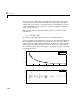
To obtain the coefficient estimates, the least squares method minimizes the
summed square of residuals. The residual for the ith data point r
i
is defined as
the difference between the observed response value y
i
and the fitted response
value , and is identified as the error associated with the data.
The summed square of residuals is given by
where n is the number of data points included in the fit and S is the sum of
squares error estimate. The supported types of least squares fitting include
• Linear least squares
• Weighted linear least squares
• Robust least squares
• Nonlinear least squares
Linear Least Squares
The Curve Fitting Toolbox uses the linear least squares method to fit a linear
model to data. A linear model is defined as an equation that is linear in the
coefficients. For example, polynomials are linear but Gaussians are not. To
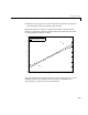
illustrate the linear least squares fitting process, suppose you have n data
points that can be modeled by a first-degree polynomial.
y
ˆ
i
r
i
y
i
y
ˆ
i
–=
residual = data – fit
Sr
i
2
i 1=
n
∑
y
i
y
ˆ
i
–()
2
i 1=
n
∑
==
yp
1
xp
2
+=