User`s guide

Parametric Fitting
3-27
Evaluating the Goodness of Fit
After fitting data with one or more models, you should evaluate the goodness
of fit. A visual examination of the fitted curve displayed in the Curve Fitting
Tool should be your first step. Beyond that, the toolbox provides these goodness
of fit measures for both linear and nonlinear parametric fits:
• Residuals
• Goodness of fit statistics
• Confidence and prediction bounds
You can group these measures into two types: graphical and numerical. The
residuals and prediction bounds are graphical measures, while the goodness of
fit statistics and confidence bounds are numerical measures.
Generally speaking, graphical measures are more beneficial than numerical
measures because they allow you to view the entire data set at once, and they
can easily display a wide range of relationships between the model and the
data. The numerical measures are more narrowly focused on a particular
aspect of the data and often try to compress that information into a single
number. In practice, depending on your data and analysis requirements, you
might need to use both types to determine the best fit.
Note that it is possible that none of your fits can be considered the best one. In
this case, it might be that you need to select a different model. Conversely, it is
also possible that all the goodness of fit measures indicate that a particular fit
is the best one. However, if your goal is to extract fitted coefficients that have
physical meaning, but your model does not reflect the physics of the data, the
resulting coefficients are useless. In this case, understanding what your data
represents and how it was measured is just as important as evaluating the
goodness of fit.
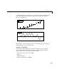
Residuals
The residuals from a fitted model are defined as the differences between the
response data and the fit to the response data at each predictor value.
residual = data - fit
You display the residuals in the Curve Fitting Tool by selecting the menu item
View->Residuals.