User`s guide

Parametric Fitting
3-33
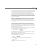
Calculating and Displaying Confidence Bounds. The confidence bounds for fitted
coefficients are given by
where b are the coefficients produced by the fit, t is the inverse of Student’s T
cumulative distribution function, and S is a vector of the diagonal elements
from the covariance matrix of the coefficient estimates, (X
T
X)
-1
s
2
. X is the
design matrix, X
T
is the transpose of X, and s
2
is the mean squared error.
Refer to the
tinv function, included with the Statistics Toolbox, for a
description of t. Refer to “Linear Least Squares” on page 3-6 for more
information about X and X
T
.
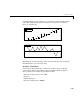
The confidence bounds are displayed in the
Results list box in the Fit Editor
using the following format.
p1 = 1.275 (1.113, 1.437)
The fitted value for the coefficient p1 is 1.275, the lower bound is 1.113, the
upper bound is 1.437, and the interval width is 0.324. By default, the
confidence level for the bounds is 95%. You can change this level to any value
with the
View->Confidence Level menu item in the Curve Fitting Tool.
You can calculate confidence intervals at the command line with the
confint
function.
Calculating and Displaying Prediction Bounds. As mentioned previously, you can
calculate prediction bounds for a new observation or for the fitted curve. In
both cases, the prediction is based on an existing fit to the data. Additionally,
the bounds can be simultaneous and measure the confidence for all predictor
values, or they can be nonsimultaneous and measure the confidence only for a
single predetermined predictor value. If you are predicting a new observation,
nonsimultaneous bounds measure the confidence that the new observation lies
within the interval given a single predictor value. Simultaneous bounds
measure the confidence that a new observation lies within the interval
regardless of the predictor value.
CbtS±=